5.1. Monte Carlo method

5.1.1. Overview

Monte-Carlo (MC) methods is a rather general term used for a variety of methods for different purposes. The methods share the approach that random numbers (samples) and the laws of probability theory are used to solve problems. The problems that are solved with MC methods in many fields, such as physics, chemistry, traffic, and economy, usually have in common that finding their analytic solution is either elaborate or impossible. They are usually hard to solve because they depend on a large number of variables that can be random or unknown to some extent. An (in)famous example is the solution of diffusion problems, as performed by Enrico Fermi and others while working on the concept of an atomic bomb at Los Alamos during world war II (Metropolis, 1987). This application represents the birth of the modern MC simulation and is also the origin of its name. “Monte-Carlo” was used as a code name that referred to the casinos of Monaco as a reference to the stochastic nature of the method (Metropolis, 1987). The MC approach is basically an application of the law of large numbers. This essential law of statistics states that when independent experiments subject to statistical variations are repeated a large number of times, the average of all outcomes converges to the expected value (Bernoulli, 1713; Poisson, 1837; Hsu and Robbins, 1947).
In the present work, only basic Monte Carlo methods are required, and only these are covered briefly here. Even though only basic MC methods are applied here, the present application is a good example of a problem that can, in fact, not be solved in an analytic way. Determining the transmitted power behind a shaded window would require solving a complex and large set of nested spatial and spectral integrals representing the relevant scattering processes and the incidence radiation. Providing the analytic solution to such an equation system is virtually impossible.
However, this task can be solved efficiently and straightforwardly by applying the MC method. Instead of considering the entire distributions that describe spectrally or angularly resolved flux densities, only single discrete samples matching the corresponding probabilities are used. These samples, which are random by nature but governed by distinct distributions, are fed as input parameters into a deterministic calculation. The results or output parameters are consequently subject to variation. However, by iterating this process for a large number of samples, the average of the results will converge to the desired expected value, and the measured variation can be used to assess the accuracy of the results. For the considered optical process, this means that the infinite number of continuous paths that energy flows follow are substituted by a large number of discrete random paths governed by probability functions.
Consequently, a key task of MC simulation is the generation of random samples that follow given probability distribution functions (PDF). Three simple methods relevant to this work are briefly presented below.

5.1.2. Simple sampling strategies

5.1.2.1. Sampling discrete values

Choosing discrete outcomes based on given probabilities represents the simplest sampling case. A good example is the determination of powers going into reflection, absorption and transmission at a scattering event. Since the relevant coefficients are determined by Fresnel’s equations and energy conservation demands that the absorption, reflection and transmittance coefficients add up to unity (𝐴 + 𝑅 + 𝑇 = 1), the MC implementation of the scattering can be performed using merely a single uniformly distributed random number:

Instead of following all paths, one distinct path is determined based on its probability and followed further on.

5.1.2.2. Sampling continuous values – inverse transform method

Provided the targeted PDF can be integrated in order to determine its cumulated distribution function (CDF) and provided this function can be inverted (CDF-1 ), a random sample following the PDF can efficiently be generated by evaluating this CDF-1 for a random number 𝑟 in the range of 0 to 1, see, e.g., (Robert and Casella, 2004):

If either the analytic integration or inversion is impossible, a numerical solution can be applied instead. However, in this case, it has to be considered that only numerically efficient solutions are suitable for application in sampling methods. A numerical inversion is, e.g., applied in this work to generate wavelength samples following the global radiation spectrum (see section 4.4.2). An analytic form of the CDF-1 function is, e.g., used to determine the z component of the diffuse reflection in the method localLambert (see section 4.11.2) or the ray starting point on a triangle (see section 7.10.2).

5.1.2.3. Sampling continuous values – rejection method

This method is applied if the CDF-1 cannot be derived analytically or if solving it is computationally too expensive, but the targeted 𝑃𝐷𝐹 𝑓(𝑥) can be evaluated for any x easily; see e.g. (Robert and Casella, 2004). In this case, an alternative 𝑃𝐷𝐹 (𝑥) that allows drawing samples based on the inversion method is applied. This function ℎ(𝑥) should form an envelope on the targeted 𝑃𝐷𝐹 function and can be scaled using a constant 𝐶 so that:

In order to achieve high performance, the function 𝐶 ∙ (𝑥) should cover 𝑓(𝑥) as narrow as possible. To determine a random sample x following the 𝑃𝐷𝐹 𝑓(𝑥) the following steps are performed:

Following this algorithm, a distribution of samples 𝑋 proportional to the target 𝑃𝐷𝐹 can be generated.
More sophisticated sampling methods include, e.g. importance sampling and the metropolis algorithm (Robert and Casella, 2004). While these sampling methods were not required in the present work, a special variant of the metropolis algorithm was used for the required optimisation processes in the thesis (see section 5.2).

5.1.3. Sampling accuracy – the central limit theorem

Apart from generating random samples, the second essential task of MC applications is to evaluate the statistical accuracy of the results. As mentioned, the Monte Carlo method relies on stochastic input parameters fed into a deterministic process producing results that are subject to variation of initially unknown scale.
In order to assess the uncertainty of the result, the fundamental central limit theorem (CLT) can be applied. The essential theorem is presented in many forms. E.g. Kreyszig et al. (2011) state it as:

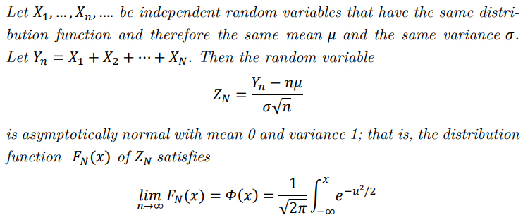
Expressed in simple words, this means that all distributions formed as a sum of distributions converge to a normal distribution centred around the expected value of all distributions. Note that the initial distributions can be of any “non-pathological” type, to put it casually, but their average, always converges to a normal distribution. More specifically, random, independent samples with finite expected values and variance are required; see e.g. Montgomery and Runger (2014).
In its practical application, subsamples of size 𝑚 of the MC results 𝑟𝑖 are used to generate 𝑛 mean values µ𝑠𝑠,𝑖 in parallel. The sample means are used to estimate the population mean µ𝑒 , that converges to the targeted expected value µ of the result (see, e.g., Montgomery et al. (2010)):

While dividing the samples into subsamples has no impact on the result of µ𝑒 , it is relevant for monitoring the accuracy of the results. Since, unlike the r𝑖 values, the µ𝑠𝑠,𝑖 will be normally distributed according to the CLT, the standard error of the sample means (𝜎𝑆𝐸𝑀) can be used to assess the accuracy of the estimate µ𝑒 . It can be derived as (see, e.g., Montgomery et al. (2010)):

This is the simple but fundamental relation used to assess the accuracy of MC results. Since based
on a normal distribution, the expression σ𝑆𝐸𝑀 can be used to state confidence intervals for the results.

one tenth, the required iterations have to be increased a hundredfold, etc. Therefore, the convergence of MC is often perceived as fast in the beginning and slow in the end (see Figure 69).