6.2. SIOP evaluation and incidence profiles
Evaluating the 𝑆𝐼𝑂𝑃 means to determine the quantity of interest 𝑞 represented by the 𝑆𝐼𝑂𝑃 for a given solar incidence profile. Based on the definition of the 𝑆𝐼𝑂𝑃 only a simple integration over the hemisphere is required for this purpose. The solar incidence profile will usually contain radiance information but could also contain time-integrated values for the radiance of unit 𝐽𝑚−2 𝑠𝑟−1 . In this case, the evaluation of the SIOP would also yield time-integrated quantities (e.g. energy instead of power). The equations derived below are valid for any type of incidence profile; however, for the sake of simplicity, the physical quantity radiance 𝐿(𝜃,𝜑) [W/(m².sr)] is used for the incidence profile. The evaluation of the target quantity 𝑞 can then be written as:

In order to perform the integration, the incidence profile in world coordinates has to be rotated into the local SIOP coordinate system according to the element’s actual orientation (e.g. a window) first (or vice versa).
In practice, a sampling method is used to evaluate the integral. As equally-spaced, discrete directions are used, the solid angle can be pulled out of the integration, which results in an elementwise multiplication. Consequently, it is possible to state the discrete integration over the entire hemisphere as:

In more general terms, the integration over any segment of the hemisphere can be formulated as:

Again, it is required that the directions 𝑗 are distributed equally spaced in the relevant segment covering the evaluated solid angle.
Rarely the angular radiance distribution on the entire hemisphere is available. Instead, a generic incidence profile can be generated based on the commonly used direct and diffuse irradiance information. In such cases, the angular incidence profile is not explicitly calculated but implicitly contained in the evaluation process. In commonly used irradiance models, the diffuse radiance is assumed constant on specific angular segments; e.g. the most simple isotropic model assumes constant radiance values for the diffuse radiation from the sky and the ground-reflected radiation. In this case, the radiance is constant in the according integration areas but generally a function of time: 𝐼(𝑡,𝑗) = 𝐼0,𝑠𝑒𝑔(𝑡). This allows to additionally pull the radiance out of the integration:

Since the term in the brackets reflects the average value 𝑆̅ 𝑞,𝑠𝑒𝑔 of the 𝑆𝐼𝑂𝑃𝑞 on a specific segment of the hemisphere, the evaluation can be written as:
Utilizing this formulation for the evaluation has a significant advantage: in order to achieve high precision, the evaluation of the 𝑆𝐼𝑂𝑃 should be performed with a large number of directional samples, which requires quite some calculation time as trigonometric functions are involved. However, if the Solar Incidence Operators Definition, generation and evaluation RadiCal, D. Rüdisser 135 radiance value is a constant for a specific fixed segment of the hemisphere, the value of 𝑆̅ 𝑞,𝑠𝑒𝑔 can be precalculated before the evaluation of the time series. Since this calculation must be performed only once, it is no longer time-critical. Consequently, any appropriate number of samples and any appropriate distribution of directions can be used for the numerical determination of the constants 𝑆̅ 𝑞,𝑠𝑒𝑔. The subsequent evaluation of irradiance time series can now be performed very fast, as it merely consists of a couple of multiplications for each diffuse component. Only for the direct solar component, an evaluation of the SIOP has to be performed on every time step. However, this can now be performed for the precise location of the sun and, therefore, requires only a single evaluation. The process is explained in detail in the following sections.
6.2.1. Evaluation with angularly resolved measured data
For the case that measured data is available with high resolution for the entire hemisphere, the full evaluation according to equations (109) or (110) can be performed using a Monte Carlo method (see section 5.1). In practice, such angular-resolved data is more likely to be available with a lower resolution (e.g. based on the Klems segmentation). In such cases, the SIOP can be evaluated by applying equation (113) for each segment that represents a locally constant (modelled or measured) radiance value. The necessary coefficients, i.e. the solid angle 𝑠𝑒𝑔 and the SIOP average value for the segment 𝑆̅ 𝑞,𝑠𝑒𝑔 can again be precomputed based on the given segmentation. This allows a fast evaluation afterwards.
6.2.2. Evaluation using a generic isotropic incidence profile
In the simple but commonly used isotropic sky model (see Hottel et al. (1942) or Loutzenhiser et al. (2007)), the solar irradiance is modelled based on three commonly used, measured (or modelled) components direct normal incidence DNI, global horizontal irradiance GHI and diffuse horizontal irradiance DHI. The model assumes that the radiance over the sky dome is constant in all directions. The model further assumes the radiance resulting from ground-reflected solar radiation is also a constant and can be modelled as a fraction of the global horizontal irradiance GHI. The relevant coefficient that determines this fraction is referred to as albedo value 𝛼. It is usually a constant representing the ground’s bi-hemispherical reflectance value. Since the model is based on the assumption of perfectly diffuse Lambert behaviour (see section 4.3.3), the radiances for the sky and ground component of the horizontally measured irradiance quantities can be derived as:
Based on these definitions, the time-series 𝑞(𝑡) for any quantity of interest represented as SIOP can easily be evaluated by applying equation (113). In addition to the two diffuse components, the direct normal irradiance is considered in a third term that evaluates the SIOP for the solar angles 𝜃(𝑡),𝜑(𝑡) (relative to the SIOP orientation):
Considering the two diffuse and the direct component, the evaluation can be written as:
The coefficients and 𝑆̅, relevant for the diffuse components, can again be precomputed, provided
that the SIOP reference system is first rotated into the correct world position.
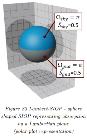
In the following, it is demonstrated how the RadiCal approach complies with the standard method by calculating the total irradiance incident on a vertically tilted plane using the 𝑆𝐼𝑂𝑃 approach. Assuming a planar, totally absorbing surface, the cosine law leads to an absorption 𝑆𝐼𝑂𝑃 that has the shape of a perfect sphere, extending to a value of 1.0 in the normal direction. It is crucial for further derivations and is hereinafter referred to as Lambert-SIOP. Its polar-plot representation is depicted in Figure 83. Following geometrical considerations, it is obvious that the precomputed coefficients for the determination of the diffuse components are:
Substituting these coefficients into equation (116), the time-dependent total irradiance on the plane 𝐸(𝑡) can be written as:

By substituting the above radiances using eq. (114), and by utilizing the fact that the Lambertian, sphere-shaped 𝑆𝐼𝑂𝑃 (see Figure 83) can also be expressed simply by 𝑐𝑜𝑠, with being the angle of incidence relative to the plane, equation (117) can be written as:
This is the standard equation used to determine the irradiance based on the isotropic sky model for a plane tilted by 90°, which has been derived consistently using the SIOP approach. Of course, the same could be shown for any other tilt angle of the plane, as the coefficients for the sky and ground term determined on a tilted 𝑆𝐼𝑂𝑃 will change accordingly.
6.2.3. Evaluation using a generic Perez incidence profile
6.2.3.1. The anisotropic Perez sky model
While the isotropic sky model is still frequently used, the assumption of constant radiance over the entire sky dome does not properly reflect the real-world irradiance profiles, leading to erroneous results. The actual radiance distribution over the sky dome and its dynamic diurnal and seasonal variation is complex. It depends on specific local meteorological conditions, in particular, of course, on the weather and cloud cover. Therefore, it is impossible to accurately describe a local irradiance situation by applying simple analytic models. Nonetheless, the isotropic model can be ‘upgraded’ by
adding additional features. In order to achieve higher accuracy, Perez et al. (1988; 1990) have identified two dominant non-isotropic components that can be modelled in an analytic way: circumsolar radiation and horizon brightening (or darkening). To be able to take local variations into account, the models are based on free parameters that can specifically be defined based on local conditions. The Perez model can, therefore, be considered a semi-empirical approach. While the direct normal irradiance and ground reflected irradiance is treated in the same way as in the isotropic sky model, the diffuse sky irradiance received by a tilted surface is now determined by (Perez et al., 1988; Perez et al., 1990):


For the application in RadiCal, it is essential to identify and separate the components of the Perez model: The first term in the square brackets of equation (119) represents the isotropic diffuse irradiance of the sky, excluding the circumsolar component. The second term, led by the coefficient 𝐹1, reflects the circumsolar component of the model, whereas the last term, led by 𝐹2, represents the horizon component of the model.
The coefficients 𝐹1 and 𝐹2 are, in turn, determined based on the irradiance components 𝐷𝐻𝐼, 𝐷𝑁𝐼, the solar zenith angle 𝜃𝑧 , as well as on the local pressure (for air mass calculation) and date, i.e. day of the year (for calculation of extraterrestrial radiation). Additionally, empirical parameters 𝑓𝑖𝑗, specific to the location, are required in the calculation process. The implementation performed here follows the often applied approach to use global values as provided in table 6 in the publication of Perez et al. (1990). The relevant parameters 𝑓𝑖𝑗 are provided in tabular form depending on the clearness parameter 𝜀, which depends on diffuse/direct irradiance ratio and the zenith angle.
6.2.3.2. SIOP evaluation using the anisotropic Perez sky model
The necessary details for the implementation of the Perez model are available in the original publications (Perez et al., 1988; Perez et al., 1990) or, e.g., on the relevant page of the PV Performance Modeling Collaborative of Sandia National Laboratories (Sandia National Laboratories, 2018b). The application of the model in RadiCal basically follows these standards with two variations: first, the determination of the coefficients 𝑓𝑖𝑗 based on the clearness parameter 𝜀 is not performed based on the discrete interval approach, as suggested. Instead, a linear interpolation method is applied (see implementation, section 6.2.5). Second, the three components forming the diffuse sky irradiance (eq. (119)) are calculated and applied separately. Based on Perez model radiance and irradiance components are defined subsequently used for the SIOP evaluation.
By following the principle of a Lambert receiver or by comparing with the equations in the previous section, the constant sky radiance value 𝐿𝑠𝑘𝑦,𝑃𝑒𝑟𝑒𝑧 can be derived from the Perez model as:

Note that this definition still considers the entire sky dome, i.e. the upper hemisphere. The horizonband introduced by Perez does not reduce its extension, as the horizon radiance values are superimposed on the sky radiance value. Since these horizon radiance values can be positive and negative, they can either increase or reduce the original sky radiance values.
For the ground-reflected component, commonly, the standard approach for the isotropic model is used. It was introduced in the previous section:

The Perez model assumes a horizon band that extends to an angle of 6.5° above the horizon. To be able to perform an evaluation analogue to the two diffuse components just introduced, a constant radiance is assumed for this region. The corresponding value for the related radiance can be found by inverting the Perez model, i.e. demanding that the irradiance evaluation of the Lambert-SIOP, representing a vertical plane, according to equation (113), has to equal the horizon irradiance component of the Perez model:
Consequently, the constant radiance value of the horizon 𝐿0,ℎ𝑜𝑟𝑖𝑧𝑜𝑛 is obtained as:

The solid angle and average value of the Lambert-SIOP used represent constants. The value for the solid angle is achieved simply by integration over the 6.5 degrees extended horizon band, considering only the hemisphere in front of the plane. The average value 𝑆̅ 0,ℎ𝑜𝑟𝑖𝑧𝑜𝑛 is obtained by evaluating the SIOP for this same region. The determined constants ensure that the irradiance values resulting from the horizon brightening (darkening) align with the original definitions of the Perez model. The actual solid angles and average values are used in the evaluation process to perform a SIOP-based evaluation of the Perez model for a plane tilted at angles other than 90° (see below). However, the constants contained in equation (122) always remain unchanged.
Next, the second anisotropic component introduced by Perez et al. is considered. In their definition, the circumsolar component represents a part of the diffuse sky radiation. This is reasonable since it Solar Incidence Operators Definition, generation and evaluation RadiCal, D. Rüdisser 139 scales with the diffuse irradiance DHI. However, for its evaluation, the sky’s clearness, which is in turn linked to the direct normal component DNI, is also relevant. Further, to calculate the irradiance resulting from the circumsolar component, Perez introduced the parameter 𝑎, which by definition is nothing but the non-negative cosine of the incidence angle (𝑚𝑎𝑥(0, 𝑐𝑜𝑠)). Hence, it is reasonable to consider the circumsolar component as directed and to handle it in the same way as the DNI component. Consequently, it is not represented as a radiance term [W/(m².sr)] but as an irradiance component [W/m²]. The related term can easily be found by replacing the parameter 𝑎 with the SIOP for the incidence direction, as the SIOP operator contains the angular profile in a more general way:

Alternatively, the SIOP operator could also be evaluated on the entire circumsolar disc as defined in Perez’ model. In future work, it will be studied if this improves the accuracy. However, the simple approach based on a singular SIOP evaluation for the circumsolar and direct component is pursued for all evaluations performed in the present work for two reasons. First, it is more in line with the commonly performed evaluation of the Perez model. Second, the single evaluation of the SIOP for the incidence angle will generally be a good estimator for the average value of the circumsolar disk centred around it.
Finally, only the direct component is missing. In analogy to the circumsolar term just derived, the irradiance resulting from direct normal irradiance 𝐷𝑁𝐼 is stated as:

6.2.3.3. Irradiance on the vertical plane – consistency with standard approach
In analogy to the derivation performed for the isotropic model in the last section, the consistency of the Perez evaluation for the SIOP is demonstrated by explicitly calculating the irradiance on a vertically oriented plane.
The solid angles for this orientation represent quarter spheres for the sky and ground component: The 6.5° extended horizon results in: ≈ 0.3556. The average values over the related SIOP segments can be determined as 𝑆̅ 𝑠𝑘𝑦 = 𝑆̅ 𝑔𝑛𝑑 = 0.5 and 𝑆̅ ℎ𝑜𝑟𝑖𝑧𝑜𝑛 ≈ 0.6353. Substituting these values into the previous equation:

For the irradiance on a plane, the evaluation of the Lambert-𝑆𝐼𝑂𝑃 for the solar position is again substituted by 𝑐𝑜𝑠. Further, equations (120) to (124) are substituted into the equation:

This, again, demonstrates that the SIOP approach transitions into the standard model for a simple planar geometry. The evaluation of equation (125) for any other orientation simply requires the (pre)calculation of the solid angles and SIOP averages applying the actual tilt angle.
6.2.3.4. Perez evaluation for a general tilt angle
6.2.3.4. Perez evaluation for a general tilt angle In order to perform the SIOP evaluation for the Perez model according to equation (127), the three solid-angle and the three SIOP average values have to be provided. All values are specific for the tiltangle and do not depend on the azimuthal, i.e. compass orientation. The solid angles represent the fractional area of the particular regions (sky, ground, horizon band) visible to an observer on the tilted plane. Following this consideration, it is evident that the areas representing the sky and ground are spherical lunes. Hence the solid angles of the visible sky (𝑠𝑘𝑦) and ground (𝑔𝑛𝑑) are simply linear functions ranging from 0 to 2𝜋 (see Figure 85) The solid-angle of the visible horizon band (ℎ𝑜𝑟𝑖𝑧𝑜𝑛) follows a slightly more complex function. For most tilt angles, it is close to 0.3556𝑠𝑟 as one half of the horizon will be visible. However, there is a slight slope, as additional wedges around the axis of rotation have to be considered. When the downwardpointing horizontal orientation is reached, the solid angle will diminish to zero as the horizon band moves out of view. In contrast, for the upright horizontal plane, the value reaches 0.7113𝑠𝑟, as the entire 6.5° extended band is visible.
While the solid angles used in the evaluation depend on the tilt angle but are generally valid for any SIOPs, the corresponding SIOP average values for the specific regions naturally depend on the actual SIOP shape. For reference and comparison with the standard model, the Lambert-SIOP, representing the irradiance on a plane, is once more evaluated. The SIOP averages as functions of tilt angle are determined by numerical integration and depicted in Figure 86. Note that the average for the horizon band (𝑆̅ ℎ𝑜𝑟𝑖𝑧𝑜𝑛) reaches its maximum when tilted slightly upwards (red arrow) and does not reach zero for the horizontal orientation (red line).
In order to analyse the impact that the radiance of each component has on the resulting irradiance on the plane, the solid angles are multiplied by the relevant SIOP averages for each component. The results are depicted in Figure 87. As can be seen, the products for the sky and ground components result in cosine- and sine-shaped functions of the

tilt angle. This corresponds perfectly to the standard Perez model, eq. (119). However, the irradiance resulting from the horizon radiance, determined by the product, follows a slightly different shape than the 𝑐𝑜𝑠𝛽 term considered in equation (119). Firstly, the maximum is offset by few degrees to the upside, which is reasonable based on geometrical considerations. Second, the impact of the horizon band radiance does not vanish for the (upright) horizontal orientation. From a geometric point of view, this is also reasonable. As stated above, the visible solid angle fraction of the horizon band increases to double the value for a horizontal plane. Even if the absorbed irradiance converges to zero for incoming light at grazing angles (according to Lambert’s cosine law), there remains a non-zero contribution of the 6.5° extended horizon band on a horizontal plane. This is an interesting deviation of the SIOP-based Perez evaluation compared to the standard model. Even if the irradiance contribution of the horizon band might be limited for a planar surface, SIOPs can generally be used to model complex structures that could, intentionally or not, absorb or redirect light coming from these directions. For such cases, it is essential to accurately consider the impact of the radiance resulting from the horizon band.

6.2.4. General approach for real-world environments
The evaluations discussed in the previous two sections assume that the view to the sky, horizon and ground is unobstructed. This represents a base case that is fundamentally important but rarely relevant for practical applications.
Following theoretical considerations, as well as the results of the full system validation performed in this work (Chapter 8), it is evident that the constant albedo approach leads to significant inaccuracies. It assumes a ground-level horizontal plane with constant Lambert reflectance (section 4.3.3). In real environments, all three assumptions generally prove to be insufficient. First, relevant surfaces in the environment generally have varying orientations and rise significantly above ground level, e.g. facades, mountains or tilted roofs. Consequently, irradiance values vary considerably for each surface, depending on its orientation and shading by other objects. Second, many surfaces exhibit significant amounts of specular reflection, e.g. metallic roofs. Finally, the reflectance will change depending on the climate and weather, e.g. vegetation surfaces change their colour and precipitation like rain or especially snow will significantly alter the reflectance of surfaces.
For practical application, individual radiance components reflected off all visible surfaces in the target’s view have to be considered. In order to do this, the geometry of these objects is mapped onto the SIOP, i.e. a segmentation of the SIOP is performed in a way that the radiance of each segment is approximately constant.
In such cases, the SIOP can be evaluated by applying equation (113) for each segment representing a locally constant (modelled or measured) radiance value. The necessary coefficients, i.e. the solid angle and the SIOP average value for the segment 𝑆̅ 𝑖 can again be precomputed based on the given segmentation. Finally, the solid angles and SIOP average values are calculated for the remaining visible regions of the sky and horizon band. These regions additionally determine if the sun is visible at its current location, i.e. if direct irradiance must be considered.
If the Perez sky model is applied for this approach, the total irradiance can be written as:


While the segmentation and evaluation of the SIOP based on the locally visible objects is a straightforward task, assigning suitable radiance values 𝐿𝑖(𝑡) to the different patches is more challenging. The time-resolved radiance values for each visible surface can be determined at various levels of detail.
Some potential approaches, ordered by increasing complexity, are:
- consideration of sky, horizon and ground radiance only, but with an arbitrarily shaped horizon line
- consideration of patches with varying albedo values (diffuse reflection, horizontal plane)
- consideration of plane irradiance on patches (diffuse reflection, oriented plane)
- consideration of plane irradiance on patches (diffuse reflection, oriented plane, shadowing)
- consideration of plane irradiance and directed reflection(direct reflection, diffuse reflection, oriented plane, shadowing)
- elaborate calculation of radiances using RadiCal raytracing and an adapted SIOP approach for the patches.
An efficient approach is currently being implemented and tested but cannot be detailed here as this would go beyond the scope of the PhD. This work focuses on the raytracing algorithm, physical optics, SIOP definition, and their validation. Future publications will, in particular, cover the handling of spatially resolved incidence profiles.
However, it is important to stress that the SIOP concept does not impose any restrictions regarding the evaluation of a detailed radiance environment. On the contrary, SIOPs in particular allow and facilitate the implementation of such angularly resolved approaches. The significant advantage of the SIOP is that radiance distributions on an arbitrarily shaped segmentation can be evaluated very accurately and efficiently.
6.2.5. Implementation Perez module
The program code relevant for the Perez evaluation are contained in the, already introduced, classes TSunposIrradiance and TRCSIOP. The latter class contains the algorithm for calculating the solid angles and SIOP average values. Both tasks are performed in the function precalcHemiMeansStdSYS :

The function samples the average SIOP values for the relevant sections of the sphere (sky, ground, horizon band) until a given precision target is met. The central limit theorem is again applied to abort the sampling at the earliest possible iteration (see section 5.1.3). In order to sample the sphere’s sections uniformly, again rejection sampling, referred to as ‘Malley’s method’ (Malley, 1988) is applied (compare section 4.11.2). This algorithm is approx. 30% faster than the standard code, which involves the evaluation of sine and cosine functions. Note that all solid angles are kept as dimensionless fractions (of quarter-spheres) by dividing them by 𝜋 𝑠𝑟.
The implementation of the Perez algorithm is contained in the class TSunposIrradiance.
The different irradiance/radiance components are provided by the function getPerezIrradiance:

The four irradiance components circumI, diffSkyI, diffHorizonI, diffGndI are calculated as described in the previous section. However, the radiance values of the diffuse components (sky, ground, horizon) are already multiplied with a factor of 𝜋 𝑠𝑟. Consequently, they are already in units of irradiance and can directly be multiplied with the dimensionless solid angles, as specified on the previous page.
The Perez parameters F1 and F2, which determine the circumsolar and horizon irradiance, can optionally be calculated based on the standard algorithm or based on the interpolated version suggested here. Only the function getPerezF1F2interpol is presented here:

As depicted in Figure 90, a piecewise linear interpolation is applied in between the centres of the clearness 𝜀 intervals defined in the standard algorithm (Perez et al., 1990; Sandia National Laboratories, 2018b). The standard Perez model’s bin number representing integer values ranging from 1 to 8 is interpreted as a real number. Linear interpolation is used to replace the discrete eight values for the 𝑓𝑥𝑥 parameters provided by Perez et al. with continuous values. The determination of the clearness index 𝜀 function getPerezF1F2interpol relies on the values of the air-mass and extraterrestrial radiation. In order to determine the extraterrestrial

radiation, the commonly used Spencer approximation (Spencer, 1971; Sandia National Laboratories, 2018a) was implemented. For performance reasons, the constants are precomputed on a daily base. The commonly used model of Kasten (1964; Kasten et al., 1989) was implemented to determine the air-mass. Both implementations are provided below:

The presented algorithms provide all the required elements for evaluating the SIOP for any given irradiance profile. The actual evaluation, representing the implementation of equation (125), is now merely a matter of a few multiplications. The full code required to finally evaluate the irradiance considering the diffuse and direct components can simply be written as:

6.2.6. Testing and validation
While many consistency and plausibility tests were carried out during the implementation of the relevant modules, an explicit two-level test for evaluating the Perez module was performed. In the first step, the validity of the Perez module, providing the individual radiance and irradiance components, was tested by calculating the time series for two different days and orientations. Afterwards, the results of the SIOP-based evaluation for horizontal and vertical orientation were computed. All results were compared against irradiance values calculated with the building performance simulation software IDA ICE (Equa S.A., 2021). The program features the Perez irradiance model and allows separate export of the irradiance components (diffuse sky, ground and direct) on different vertical planes and the horizontal plane (“roof”).
Measured high-resolution (1 second time steps) irradiance values of the local weather station for two days were used as input data. The first day (14.6.2021) had a clear sky, while the second (17.7.2021) was mostly overcast. The location of the weather station is the rooftop of the AEE INTEC laboratory in Gleisdorf (latitude: 47.1097°, longitude: 15.7096°, altitude: 369 m). The albedo value was set to 10% in both calculations.
6.2.6.1. Validation of Perez module – comparison of diffuse components
First, the correct implementation of the Perez algorithm was tested. For this purpose, the diffuse sky components, and additionally the ground component, were compared. According to the Perez model, the diffuse sky irradiance depends on several parameters in a complex way, including direct normal irradiance and day-of-year. Consequently, comparing computed diffuse irradiance time series for different orientations represents a comprehensive and robust validation of the algorithms involved.
Since the RadiCal implementation contains an additional, optional interpolation feature, two calculations were tested. The results of the validation are shown in Figure 91.

The comparison of the diffuse sky irradiance time series shows an excellent agreement between the RadiCal and IDA ICE calculations. The coefficients of determinations and errors are listed in Table 12. As can be seen, the calculation results are mostly identical. The singular, relatively high maximum error for the horizontal is likely caused by the different handling of time frames in connection with the strong short-term fluctuations. The irradiance data measured in one-second intervals have to be averaged to minute intervals. Since obviously different averaging methods or different reference times are applied here, strong short-term irradiance fluctuations lead to a deviation in the results. The small values for the mean error indicate this, as the fluctuations average out when mean values are calculated.

It is also apparent that the interpolation feature of RadiCal has no significant impact on the comparison regarding average errors or correlation. Nevertheless, the feature leads to noticeable smoothing. Albeit the quantitative effect is small, this represents an appropriate improvement of the calculation, as it leads to a more realistic dynamic behaviour. It removes the transient, step-like changes, benefiting dynamic thermal simulations. Figure 92 shows a zoomed detail of the comparison. It can be seen that the standard Perez model (grey) leads to step-like changes in the diffuse irradiance, whereas the interpolation feature leads to an unbiased, smoothed curve.

6.2.6.2. Validation of SIOP evaluation vs. IDA ICE calculation
In this next step, the entire SIOP evaluation process is validated. Again, the Lambert-SIOP (see Figure 83) representing a planar absorber is used. Also, the same days as for the previous steps are used for the evaluation. The tests are performed for three vertical orientations (south, west, north) and the horizontal plane.
The results of the evaluation are presented in Figure 93, Figure 94 and Table 13.


It can be seen in the charts of Figure 93 and particularly Figure 94 that there are noise-like deviations at times with strongly fluctuating irradiance values. As mentioned in the previous section, these deviations are the results of different averaging processes or different time-frames used to generate minute interval data of the original measurement data with one-second time steps. This is confirmed by the mean errors (Table 13), as they show no significant bias. Apart from the fluctuations, the calculated irradiance values show an almost perfect match (see Figure 93 and Figure 94 – dashed red curve overlapping grey curve). The only significant systematic deviation can be found in the case north, 14.6.2021 (see Figure 93, bottom left). A systematic deviation of approximately 5 W/m² Solar Incidence Operators Definition, generation and evaluation RadiCal, D. Rüdisser 153 occurs in the morning and -9 W/m² in the evening. Surprisingly, the direct normal irradiance components differ at these times. The results of the RadiCal implementation were cross-checked by comparison with the standard Perez model, where no error was detected. The reason for the deviating calculation of IDA ICE remains unclear. As the solar positions calculated were found to be almost identical, only a minor tilt of the northern plane could potentially explain the occurring deviation.
6.2.6.3. Validation of Lambert-SIOP evaluation vs. standard on-plane irradiance model
In a further validation step, the SIOP evaluation results for the Lambert-SIOP were compared with on-plane irradiance calculations using the Perez method. For the latter, the RadiCal Perez module was used, as this module has already been validated against the IDA ICE calculations in the first step (see above). As both calculations can now be performed using the same time frames, no sampling-related noise is affecting the comparison. The results of both calculations were found to be virtually identical, showing average deviations in the range of a few thousandths Watt per square metre. Consequently, the results are not presented in graphical form. The comparison of the LambertSIOP evaluation vs. the standard Perez algorithm seems trivial. Still, it is a robust and comprehensive proof of the implementation’s validity, as the two calculation paths differ significantly. While the standard calculation is based on trigonometric functions of the tilt angle and solar angle, the SIOP evaluation is based on numerical integrations and vector calculus. The perfect match of the resulting irradiance on planes with different orientations confirms, in particular, the validity of these evaluation steps:
- generation of SIOP
- evaluation of SIOP (for singular direction)
- integration on SIOP over segments (for average values)
- calculation of solid angles of segments (sky, horizon, ground)
- determination of radiance values for segments
- two-axis rotation into the world coordinate system