7.4.1. Line triangle intersection

Only the line-triangle intersection algorithm is applied in the implementation, as already triangulated geometry is used. Models that do contain quad faces (consisting of four points in a plane) can trivially be split into two triangles for the test. There are many different approaches for calculating the intersection point. In the current implementation, the Müller-Trumbore algorithm (Möller and Trumbore, 1997) is applied. The test, on the one hand, has a high algorithmic efficiency and, on the other hand, can already provide essential information regarding the location of the intersection point relative to the ray origin point and in the coordinates of the face hit.
As can be seen in the implementation below, the algorithm is quite short if vector notation is used.

The parameters ray origin point (rayP0) and direction (rayDir) as well as the face (Tri) are passed as input to the function. The function is of boolean type and returns false if the triangle is missed. Otherwise, it returns true and passes the intersection point in world coordinates (ipoint) as well as Figure 97 Collision detection to determine intersection point closest to ray origin (𝑃0 ⃗ ) in direction 𝑑 A full spectral polarisation Monte-Carlo Raytracer RadiCal, D. Rüdisser 160 in barycentric coordinates of the triangle forming the face (u_,v_). Beyond that, it outputs the parameter t that contains the distance between the ray origin and the intersection point. This information is crucial to determine the closest collision point along the ray’s path and to avoid unnecessary calculations for further distances. As can be seen in the code, a part of the efficiency of the algorithms results from the integrated early termination tests. At various points, the execution is aborted if the current calculation results no longer allow an intersection.

The latter two show significantly higher performance. While the actual performance depends on the specifics of the geometric model, a slightly higher performance can be expected of the kd-tree for many models (Szirmay-Kalos et al., 2002). However, since the octree method is less complex to implement and the performance difference is limited, the octree method was implemented here. It can easily be replaced or extended with other methods later on.
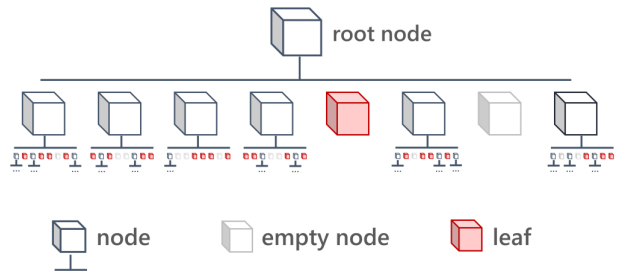
The implemented octree method is based on the initial ideas by Meagher (1980) and many further implementations. The algorithm was, however, implemented from scratch for the RadiCal method, applying today’s available modern programming features such as object-oriented programming and dynamic memory allocation. The method begins with a bounding box containing the entire model. This root box is then recursively subdivided into eight equally sized sub-boxes, and the number of faces contained in each sub-box is analysed. The subdivision is carried on recursively if the face count lies above a certain threshold. Otherwise, the subdivision is aborted, and a list with indices of the contained faces is created for the last element. As commonly applied for search trees, all elements containing face lists are referred to as “leafs”, while all elements that refer to child boxes are referred to as “nodes” (see Figure 109). Both elements, contain the coordinates of the associated bounding box.

There are mainly two advantages resulting from this partitioning. First, the nested hierarchy efficiently excludes large parts of the model if the bounding boxes of higher-level nodes do not intersect with the ray. Second, the required box-line intersection tests, which are always performed before the final face intersection tests, can be performed very fast, as the rectangular bounding boxes are aligned to the axis of the coordinate system. More considerations regarding the algorithm can be found in Meagher’s original publication (1980).
A customized implementation has been written for use in the raytracer. It is contained in the class TFaceTree of the module rc_facetree.

There are essentially only two functions relevant for the application of the module: createTree and nextRayCollRecursive. The first one is used to establish the octree. For this purpose, the geometry (geo_) and root bounding box (bb0) are passed to the module. In order to control the tree generation, the maximum number of faces per leaf is provided (maxLeafSize). During the implementation, two additional features were implemented and found to be useful for increasing the performance on some geometries: minDim_ allows defining a secondary recursion abortion criterion based on the volume of the bounding box. Finally, the isoScale parameters can be used to transform the root box into a cube. If this option is not chosen, the proportions of the initial bounding box will be maintained throughout the recursion. Since the tree generation can take up several minutes, the functions saveToFile and readFromFile can be used to store and reuse an already generated hierarchy.
Finally, the function nextRayCollRecursive is the key function that performs the collision tests in the raytracing process. In the exceptional case of not detecting any collisions, it returns false; otherwise, it updates the currColl variable in the ray parameter with specific information regarding the detected collision. As shown in section 7.3.1, the collision structure contains comprehensive information for the face hit. Most of these parameters are provided by nextRayCollRecursive already. This increases the performance of the raytracing, as calculations results from the triangle intersection can be used for this purpose. Specifically, the following parameters of currColl are provided: