Müller matrix operations

4.9.1. Background and theory

Since the Stokes representation uses a 4D vector to describe the polarisation state, a 4×4 matrix can be used to model scattering events that alter the polarisation state of the beam. Generally, these matrices are referred to as Müller matrices (after Hans Müller, who introduced them in 1943). Müller matrices are primarily used for evaluating empirical data gathered with optical methods (e.g. by ellipsometry) or for designing optical systems when polarisation effects have to be considered. In such cases, the polarisation properties of the optical elements used (e.g. linear polariser) are characterised by their specific Müller matrices.
For the RadiCal raytracer, currently, only two Müller matrices are relevant. However, these are able to cover a wide range of polarisations effects as the implemented, generalized approach for computing the Fresnel coefficients (see section 4.7.1) also provides information for the phase change occurring on the scattering event (𝝐𝒑, 𝝐𝒔). The two implemented Müller matrices are used to calculate the polarisation states, as well as the intrinsically contained powers of the (specularly) reflected and transmitted beam at interfaces of materials. Additionally, coatings (e.g. low-E, antireflective) or naturally occurring thin-films (e.g. oxide layers) can be considered, as they can be modelled with the implemented approach to determine the generalized Fresnel coefficients and resulting phase shifts. In general, the reflection of an unpolarised beam on a surface will lead to a transmitted and reflected beam. The polarisation state, as well as the intensities of the incident, the reflected and transmitted beam are described by their Stokes vectors 𝑆 𝑖 , 𝑆 𝑟 and 𝑆 𝑡 .

Using the Müller matrix for reflection 𝑀̅𝑟 , the Stokes vector of the reflected beam 𝑆 𝑟 , based on the generalized Fresnel coefficients (see eq. (53) and (54)) can be found by:

Likewise, by using the Müller matrix for transmission 𝑀̅𝑡 , the Stokes vector of the transmitted beam 𝑆 𝑡 is determined by:

The Müller matrices 𝑀̅𝑟 and 𝑀̅𝑡 are a function of wavelength and incidence angle, as the generalized Fresnel coefficients used to calculate them are so. Consequently, they have to be computed individually for each scattering event.
While in the above formulation of the Müller matrix, the explicit dependence of the phase angles and amplitudes is easily accessible, an alternative formulation of the Matrix based on the complex amplitudes 𝑟̃and 𝑡̃allows a computationally more efficient evaluation.

The phase information is now contained in the complex-valued amplitudes. Hence, these alternative formulations of the Müller matrices do not rely on computationally expensive trigonometric functions (sine and cosine). Further, the explicit determination of the phase-angles (see (54)) can also be omitted now. This additionally increases the algorithm’s performance, as the explicit evaluation of the two phase-angles requires the computationally expensive use of the arctangent function.
By definition, the generalized Fresnel coefficients are only valid for radiation polarised strictly parallel (𝑅𝑝, 𝑇𝑝) and perpendicular (𝑅𝑠 , 𝑇𝑠) to the plane defined by the surface normal and the propagation direction. Hence, the Stokes vector for the incident radiation, defined for an arbitrary orthogonal coordinate system 𝑝 ′ , 𝑠 ′ , has to be provided in the aligned coordinate system 𝑝 , 𝑠 determined by the surface’s normal vector 𝑛⃗ (see Figure 35). To perform this, the Stokes vector has to be transformed accordingly. After the corresponding (clockwise) rotation angle 𝜑 is determined, the aligned Stokes vector 𝑆 can simply be calculated by:

The rotation matrix 𝑅(𝜑) is not referred to as Müller matrix here, as the actual polarisation state
and the total intensity of the Stokes vector are invariant to this transformation. Solely the reference
coordinate system of the Stokes vector is rotated.

4.9.2. Implementation

In the implementation, the Müller matrix class TMuMatModule in the library rc_mumat has been chosen to encapsulate all data and classes needed to perform the Fresnel and Stokes operations relevant for a specific material interface.

As can be seen in the header, one instance of the TFresnel class (containing the methods to perform the Fresnel calculations), as well as several instances of TRIbaseclass (containing the material data), are included and used within the TMuMatModule class.
While the methods getExplicitMuMatR and getExplicitMuMatT are used for validation purposes, the raytracer solely calls the key method getMuMatRTangle, which performs all necessary operations to finally provide the Stokes vectors for the reflected and transmitted beam. The method only performs the matrix multiplications (equations (62) and (63)) and, in turn, calls the method stokesCalcRT to get the required values for the Müller matrices in the form of a TTRpolRecord. As mentioned above, the necessary parameters for the evaluation of the Müller matrices are provided in complex-valued form. Further, to avoid redundant calculation and minimize the calculation time, the functions getMuMatRTangle and stokesCalcRT pass additional parameters of the Fresnel calculations relevant for the raytracing process (see inline comments in the source):

4.9.3. Testing and validation

While the standard tests during implementation have been performed with due care, extended validation tests were performed to ensure the validity and functionality of the implemented code. The calculation of the outgoing Stokes vectors by multiplication with the corresponding Müller matrices is trivial. However, the determination of the Müller matrices depends fundamentally on the material module TRIbaseclass and particularly on the TFresnel module, which provides the necessary coefficients. Hence, the following examples prove the validity of all three modules.
As mentioned above, the detailed modelling of optics considering polarisation is currently mainly applied for advanced instrument design, astronomy and optical measurement systems (e.g. ellipsometry). Therefore the following examples are mainly of these fields. The complexity of the following validation cases gradually increases.

4.9.3.1. Validation Case 1 – Simple Silver Mirror
[constant wavelength, constant angle, no thin-films)]

This example has been found in a working paper by Tetsu Anan (2018) in which he evaluates the validity of calculations performed with the Zemax OpticsStudio software, which is widely used for advanced optical instrumentation design and also offers polarimetric raytracing features. In the paper, the Müller matrix of a reflection on a 45° tilted mirror is calculated. The precise wavelength and refractive index are provided in the example (see Figure 36).
In order to demonstrate how compact the validation can be done based on the implemented libraries, the entire source code is provided here:

The resulting Müller matrix for reflection is:

Considering the number of digits provided, the result perfectly matches the Zemax calculation results and Anan’s verification thereof (see Figure 36).

4.9.3.2. Validation Case 2 – Aluminium mirror with an oxide layer
[constant wavelength, variable angles, thin-film]

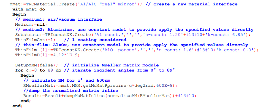
In a publication by van Harten et al. (2009) the polarisation properties of a “real mirror” are modelled using the Müller matrix and thin-film approach as applied in RadiCal. In the paper, the effect of the (usually present) amorphous aluminium oxide layer and its thickness is investigated.
Again, the complex refractive index values for the bulk material (Aluminium: 𝑛̃ = 1.2 − 6.85𝑖) and the thin-film (Aluminium oxide: 𝑛̃ = 1.6 − 0𝑖) is provided as a constant value for the wavelength used (600 nm).
The thickness of the oxide layer of the final mirror was determined as 𝑑 = 4.12𝑛𝑚.
These parameters were used for the implementation of the model with RadiCal. The entire source code used for the validation is provided for this example as well:

Since van Harten et al. have provided the Müller matrix elements in a commonly used table of charts representation, it is possible compare the results for the six non-zero matrix elements. For this purpose, the RadiCal calculation results are superimposed on the original charts. The red curves and grid lines represent the results of the RadiCal calculation; the black and grey elements are the original data of the publication.

As can be seen, the RadiCal calculations show a perfect match with the calculations of van Harten et al.. Further. it is evident (see elements m12 and m21 in Figure 37) that the ability to include thinfilms increases the potential and accuracy of the model considerably (compare grey curve vs. red/black curves and dots in Figure 37).

4.9.3.3. Validation Case 3 – A space mirror (Sciamatchy on Envisat)
[wavelength range, two angles, two layer thin-film]

In their publication ‘Mirror contamination in space I: mirror modelling’ J.Krijger et al. (2014) have extended the approach of van Harten et al. (2009) by assuming an additional contamination layer in the form of an oil thin-film. The new model should be able to better predict the mirror’s reflectance in the UV-range, where the simple model by van Harten showed the largest deviations. Based on their two-film model (oil and oxide), they provide reflectance data for the mirror for two angles of incidence and in a wavelength range from 300 nm to 1500 nm. The modelled data is compared against measurements performed by ESA for the calibration of the aluminium scan mirror of the Sciamatchy spectrometer of the Envisat satellite.
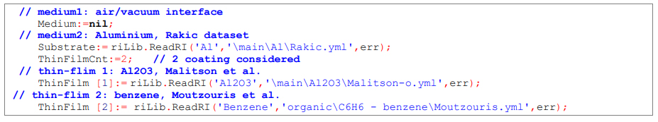
Since they do not provide the entire information regarding the refractive index functions for oil, the amorphous aluminium oxide and the bulk aluminium in the relevant wavelength range, the RadiCal implementation is used to redo the work performed in the paper, i.e. based on the given refractive index functions, the optimal thin-film thicknesses for the two-layer model is determined. This approach also allows testing the TRIClasses used to import refractive index information from external sources. The datasets of Rakic (1995) for Aluminum, Malitson et al. (1958)for Al2O3 and Moutzouris et al. (2014) for benzene (based on corresponding RefractiveIndex.INFO (Polyanskiy, 2022) database files) were applied.
Only the implementation of the material definition, based on the imported datasets, is shown below:

Of course, whether the chosen refractive index functions match the real thin-film properties is debatable, as thin-films of only a few nanometers usually show deviations from the behaviour of the Light, sun and optics – applied principles, models and methods RadiCal, D. Rüdisser 76 bulk material. However, this argument is also relevant to the assumptions regarding refractive index and layering in the publication by Krijger et al..
After optimisation, the surprisingly best fitting result, measured by the average RMS of all data points, is a thickness of 𝑑 = 5.3 𝑛𝑚 for the oil film and the elimination (𝑑 = 0 𝑛𝑚) of the oxide layer. The dispersion curves of both thin-films are of similar shape; however, benzene shows a steeper rise of the refractive index towards the UV wavelengths, which seems to lead to better results in this region. Physically, the 5.3 nm thin-film of benzene represents the single layer of contaminated aluminium oxide but is not an actual homogeneous oil film.

Again, the original chart is used to superimpose the data computed with RadiCal. As is shown in Figure 38, the results of the presented model match the results of Krijger et al. for wavelengths greater than 500 nm. Due to the different choices of film thickness and the different refractive index datasets, deviations can be seen in the UV range (300 nm measurement). While the S-61° measurement shows a good match, the other model results at 300 nm show a slight deviation to the upside, while the Krijger model generally shows deviations of the same scope to the downside.
The validation case proves that the RadiCal method is implemented correctly and able to perform advanced optical calculations, as applied in space technology.

Again, the original chart is presented, and the RadiCal calculation results are superimposed on it (see Figure 39). The results perfectly match the original calculations of Jellison. As can be seen, the characteristic variation of the ellipsometric angles  and  allows a very precise determination of the thin-flim layer thickness from 0 up to a thickness of 283 nm. For higher thicknesses, the results will be cyclically mapped on the same graph with a modulo of that value.

4.9.3.5. Validation Case 5 – Ellipsometric measurements with variable angles
[thin-film with variable thickness and incidence angles, ellipsometry]

In their publication ‘The influences of roughness on film thickness measurements by Mueller matrix ellipsometry’ Ramsey and Ludema (1994) have conducted research on the effect or layer thickness and roughness of various materials using a dual rotating-compensator Mueller matrix ellipsometer.

The measured data for the Müller matrix elements of three different angles of incidence and the angular variation of the elliptic angles for steel samples with five different coatings is replicated by performing “virtual ellipsometric measurements” using the RadiCal libraries. The computed data is then compared against the measurement data. The data of the five polished steel specimens 1A -1E coated with variable thickness of magnesium fluoride (MgF2) was used for this comparison. The wavelength of the laser (632.8 nm), the incidence angles as well as the complex index of refraction values of the materials (steel: 𝑛̃ = 2.501 − 3.408𝑖, MgF2: 𝑛̃ = 1.38 − 0𝑖) were defined in line with the parameters stated in the publication.
First, the full Müller matrix is calculated and compared for the steel sample coated with 315 nm MgF2. The publication provides measured matrix elements for three different incidence angles. The original measured data, computed data and absolute deviation are presented in Table 7.

The comparison of the ellipsometric angle functions reveals a remarkably high level of agreement with the measured data (see Figure 41) as the ellipsometric angles are usually very sensitive to small changes of the influencing parameters (i.e. layer thickness, refractive indices, incidence angle).