7.10. Directional scanning process

7.10.1. Overview

In the directional scanning process, the scattering characteristic of the target object is determined for various target quantities. For the applications addressed by this work, the target quantities will mostly be the power absorbed in various elements of the object as well as the power transmitted through the target object. Based on the principle of the linearity of light (see section 4.2.2), it is possible to capture the optical behaviour of the target object using parallel beams of light coming from different directions. This angularly resolved information can later be superimposed to determine the target quantities for any given radiance profile (see section 6.2).
Technically, the scanning process can be characterised as a Monte-Carlo forward raytracing process. This means that random rays, or light particles, are cast according to their actual direction of propagation. Following the Monte-Carlo approach, the wavelengths of the cast rays as well as all physical models governing the absorption and scattering of light are modelled as stochastic processes, i.e. random samples representing the underlying physics are used throughout to model all processes. In line with the Monte-Carlo approach, the raytracing process is iterated for a large number of samples, and the resulting mean values of the target quantities and their standard deviations are tracked. By applying the central limit theorem, see equation (91), these values can be used to determine the required number of iterations for achieving the results with specified precision.

An overview of the process is depicted in Figure 106. Essentially, the process involves the following steps:
1. A distinct direction of the incidence beam is determined using the Fibonacci hemisphere (section 5.1). A large number of rays/light particles are defined. Their wavelengths are determined based on the global radiation spectrum (see section 4.4), or any other given spectral density function. Their initial polarisation state is generally defined as unpolarised, but can also be set to a specific polarisation state.
2. The equienergetic light particles are cast from a caster object to impact the target with a specified and uniform flux density (see below).
3. The light particles are scattered, i.e. reflected or absorbed, on the surfaces of the target object. All scattering processes follow Monte-Carlo implementations of physical-opticsbased models (chapter 2). The particles always maintain their full initial energy (or flux density), or, in other words, the path of the light ray is not branched into different subpaths. Instead, at any scattering event that partially absorbs or reflects a ray, one potential outcome is chosen following the probability distributions of the underlying physical processes.
4. Since equienergetic particles are used throughout the process, the powers absorbed, reflected or transmitted by specific surfaces of the target objects can be determined merely by counting the particles. These values provide essential information for later modelling of the energy balance of the analysed object.
5. A catcher object finally captures any rays that are transmitted through the target object. The catcher object can be seen as an ideally black surface that absorbs any light particles. However, due to its virtual nature, the power absorbed by the catcher is considered a transmitted power. Alternatively, a set of catcher surfaces can be used to capture the transmitted power’s directional distribution (e.g. by again using the Fibonacci Hemisphere or a Klems segmentation).

7.10.2. Caster/Catcher concept

7.10.2.1. The caster concept

In the raytracing scanning process, the target is illuminated by parallel light beams coming from all sampling directions. In the raytracing approach, parallel light beams are represented by rays from randomly evenly distributed starting points with the same directional vector. The starting point distribution has to fulfil two criteria: first, the origin points must be uniformly distributed on a plane perpendicular to the direction with a predefined density. Second, the location of the starting points should guarantee that all relevant surfaces of the target are hit, but only a few, or in the best case, none, should miss the targeted area.
In order to achieve these goals efficiently, the caster concept was conceived. The caster represents an object that wraps around the targeted area of the target object. The caster object can be of random geometry as long as it fulfils certain criteria:

• the entire target area has to be covered
• the target area, together with the caster object has to form a closed object
• the caster object has to be convex so that it will not block itself, i.e. rays cast from any faces of the caster object that potentially hit the target area will not be obstructed by other faces of the caster.
• for identification, the object should be named “CASTER” in the CAD model.
• the surface normals of the faces that constitute the caster have to point towards the target, i.e. towards the inside of the caster object.

Some potential geometries of caster objects are depicted in Figure 107.

7.10.2.2. Generating starting points on the caster surface

As discussed above, the task is to generate randomly distributed starting points on the caster so that the associated flux density perpendicular to this direction is uniform and matches a defined value. Following these criteria and in the context of the MC approach, this transforms into two stochastic tasks:

1. face-sampling: randomly determine a face of the caster object
2. point-sampling: randomly choose a starting point on the face

In order to pick a random face efficiently, some auxiliary variables are determined before the distribution is generated. First, the probability of selecting a specific face 𝑖, with surface normal 𝑛⃗ 𝑖 and area 𝐴𝑖 is calculated. The probability for this face is determined by the radiant flux Φ𝑖 (or radiant power) that the face contributes to achieving a constant flux density 𝐸 in the specific direction 𝑣 :

As 𝐸 is constant for all faces, the probability of selecting a face is proportional to the weighted projected area, or in this case more accurately, the projecting area of the face. The maximum function ensures that only faces pointing towards the direction of the light are considered. Using equation (130), the radiant fluxes are calculated for all faces forming the caster. The results are cumulated successively in an array. In the actual implementation, however, already the proportional quantity, density of rays per watt and square metre, denoted as 𝑃, is considered:

Based on these definitions for 𝑢 and 𝑣, a uniformly sampled point on the triangle can be found by using equation (131) again. Both sampling algorithms have been tested by using different caster geometries and analysing the uniform distribution of the rays when projected on a screen.

7.10.2.3. The catcher object

The concept is completed by a second complementary object that is used to catch any rays not absorbed by the target object. The requirements for this object are, however, less complex. Actually, the only criterion is that it should wrap the geometry so that it can absorb any rays that were not absorbed by the target or the caster object. Of course, the catcher object should not penetrate or interfere with the target object or caster in a way that it captures rays that are still relevant for the raytracing process. Again, the face normals of the catcher object in the CAD model should be oriented inwards. The distinct face orientation allows raising warnings in case the catcher object is hit from the outside, which would then indicate an error in the geometry or raytracing process.

7.10.3. Incidence beam – starting a ray

The direction of the incidence beam is determined based on the chosen method: the N discrete sampling directions can either be provided by a Fibonacci hemisphere (see section 5.3) or, alternatively, by the Klems segmentation. On every iteration, the given direction is provided to a method called StartRayDir, which initialises the remaining parameters that are required to start a ray (light particle). The following steps are required to launch a single ray:
1. Determine starting point
This is done based on the algorithms explained in the preceding chapter (see 7.10.2). Firstly, a subsurface of the caster object is determined, and then a random point on the face is picked.
2. Initialise wavelength
In the standard process, the function getSampleWLat (see 4.4.2) is called to generate a random wavelength sample based on the global radiation spectrum. Alternatively, for special applications, any other spectral distribution could be considered. Beyond that, the scanning process could also be performed for monochromatic samples, particularly for three wavelengths representing the (R, G, B) values for lighting applications.
3. Initialise polarisation state
For most applications, the polarisation state will be set to the unpolarised Stokes vector (see Table 6). Again, alternative definitions for other application fields are possible (e.g. for performing virtual ellipsometric measurements, see, e.g. validation examples in section 4.9.3). Further, the polarisation reference system has to be initialised by providing an axis for spolarisation. In the case of unpolarised radiation, the axis can be randomly chosen but has to be defined perpendicular to the direction of light.
4. Initialise absorption coefficient
The volume absorption coefficient has to be provided for the first path of the light particle after its creation. Later this information will be provided by the light-surface interaction modules. Since no atmospheric absorption is considered and the rays will usually be launched in the air medium, the value is initially set to zero.
5. Initialise collision trackers
The trackers for the current and recent collision points have to be initialised. While the recent collision is defined as unset, the current collision point references the relevant surface of the caster object. This is necessary to exclude the starting surface from the first collision detection cycle. Otherwise, the starting face could be erroneously detected as the first collision.
The implementation of the ray initialisation routine is provided in full in the code snippet below. The initialisation steps are carried out in the same order as specified above.

7.10.4. Measurement of target quantities

In order to provide a versatile method to perform measurements in the raytracing scan, measurement functions can be assigned based on the surface’s material assignment. This allows a flexible approach, as the user can freely define measurement regions on any object by assigning specific materials. While these materials can still be based on identical physical properties, the separation allows for performing individual measurements. Currently, only energetically relevant measurement functions are implemented. However, the evaluation of other quantities, such as degree of polarisation, angle of polarisation or spectral properties, can easily be added in future.
The intended measurements are defined in the initialisation of the scanning process using the function addPowerMeasurement. The function tracks the absorbed, transmitted or reflected power for either a single material or cumulated for two different materials. The data is stored as an array for all N directions of the scanning process. Later on, this sampled data is used to generate the SIOP (see section 6.1.2).
Each measurement is initialised by providing the following arguments for the addPowerMeasurement function:

• mId[1,2] The material identifier is used to assign the measurement function to a specific material. If the value -1 is passed for the second material, only one material is considered in the measurement.
• lsiType[1,2] Specifies the “light-surface-interaction” type that should be measured. The options lsiAbsorbed, lsiTransmitted or lsiReflected are used in order to determine which power should be tracked on the material.
• inciType[1,2]This parameter is used to specify the incidence direction for the measurements. If itFront or itBack is selected, only hits from either the frontside or backside will be considered. If itBoth is chosen, all hits of the surfaces are tracked.
• referenceArea
  A reference area can be provided to convert the measured powers into irradiance (flux density) values [W/m²]. If no reference area is provided, the results are considered to be of type power [W].
• filename
  Finally, a filename for the sampled measured data is provided. The measured data, along
  with specifications regarding the scanning process, are stored in the specified file.

The function can best be explained with the help of an example. Below is a typical example for the initialisation of measurements used to evaluate the performance of a shaded window detail.

probe area, as the material of the probe area is defined as TLSISidealTransparent (see Table 14). However, the type lsiAbsorbed is used for the internal absorber object (catcher), as its material is defined as TLSISidealBlack. Both measurements, however, are actually used to determine transmitted radiation. This approach ensures that the probe can be used for measurements restricted to a specific region but does not distort the results of the internal absorber. Furthermore, both types are limited to frontside incidence using the itFront specifier, as no incidence from the backside is expected.
In order to determine the absorption of the three window panes and slates, the specifier lsiAbsorbed is used. To further consider the absorption of any incidence direction, the specifier itBoth is chosen. While the slats are defined using a single material, two materials are used for each glass pane. In the example, the absorptions on each side of the panes are cumulated into one measurement by referencing the materials of both sides within a single measurement (PANE1_e and PANE1_i etc.). While the provided example is kept simple, the material-based measurement concept can be used to perform refined measurements in specific areas, e.g. distinct parts of the window frame or segmented or stratified regions of the glazing.

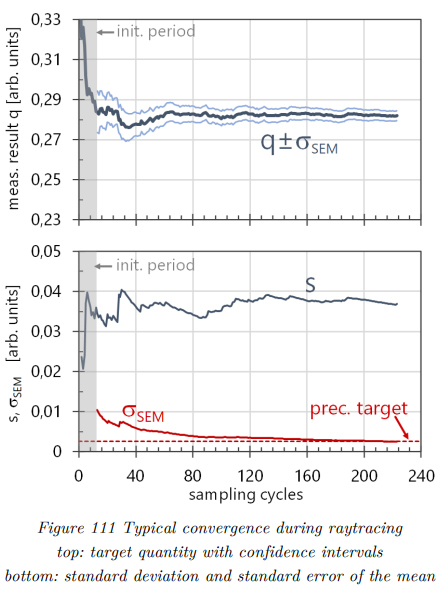
As discussed in section 5.1.3 the error estimators are derived from sampled means values. In order to achieve this, mean values of cycles with constant numbers of iterations are tracked. In the example depicted in Figure 111, each sampling cycle consists of 10,000 single raytracing processes. After each cycle, the mean value of all cycle results (𝑞) and the standard deviation (𝑠) are computed. Finally, equation (91) is used to evaluate the standard error of the mean σ𝑆𝐸𝑀, which is then compared against the precision target. The iteration is terminated if it falls below this threshold for four consecutive cycles. In the example provided in Figure 111, the precision target of 0.0025 was reached after 230 cycles, equivalent to 2.300.000 million single raytracing processes. A false, early termination can be triggered during the first few cycles when the statistical evaluation is still unreliable. In order to prevent this, the error tracking is suspended for an initial period with a constant number of iterations.