Nature of light

4.2.1. Relevant spectral ranges and definition of “light”

For technical applications, it is a widespread convention to use the term “light” to refer to the visible light spectrum and “solar radiation” to refer to the entire global radiation spectrum. For the sake of readability, the more general convention is followed here: the term “light” is used to refer to the entire global radiation spectrum comprising ultraviolet, visible and near-infrared radiation (NIR), while the term “visible light” is used to exclude the non-visible spectral ranges explicitly.

Following another commonly used convention, the global radiation spectrum is limited to the spectral range from 300 nm to 2500 nm. While extraterrestrial radiation still comprises approx. 3% of the total power above the threshold of 2500 nm, most of it is absorbed in the atmosphere by water vapour and CO2 molecules, and, therefore, is not relevant. Compliant with the applicable standards (see e.g. EN 410, 2011), visible light is defined in the present work as radiation with a wavelength ranging from 380 nm to 780 nm.
Figure 11 gives an overview of the lower half of the global radiation spectrum and the relevant wavelength range definitions. It also shows the spectral tristimulus functions relevant to the perception of colours, as defined within the standard CIE 1931 (CIE – International Commission on Illumintation, 1931). The bottom chart depicts the photopic luminous efficiency function that describes the overall sensitivity of the eye to light. Further, it contains the melanopic efficiency function (International Well Building Institute, 2022). It describes the sensitivity of melanopsin photoreceptors to light, which is highly important for the body’s circadian (day/night) rhythm. More detailed information on the global radiation spectrum is contained in section 4.4.

4.2.2. Linearity of light

Throughout this work, linearity of light is assumed, implying that light waves will not interact, i.e. light beams can cross without influencing each other. The superposition principle is a direct consequence of this linearity. It implies that two wave-functions 𝐸1 and 𝐸2 satisfying Maxwell’s equations can simply be added to find their superposition 𝐸𝑡𝑜𝑡, which will itself be a solution of Maxwell’s equations, i.e. it will satisfy the derived wave equation, see (31):

For completeness, it should be added that nonlinear effects can even be observed in the absence of matter, i.e. in a vacuum. However, these effects are again significantly weaker and can only be explained based on quantum electrodynamics. For the practical application of the presented method, linearity and the resulting principle of superposition is essential as it allows decomposing radiation processes in space, angularly, spectrally, as well as in time. Conversely, the individual components can later be superimposed in the evaluation process, considering any specific angular irradiance profiles or time frames.

4.2.3. Coherence and interference

Coherence is an ideal property of waves allowing them to form stationary, or quasi-stationary, interference patterns in space or in time. In the present work, coherent as well as non-coherent superposition of light beams are assumed for modelling different processes. While this may sound inconsistent at first, it is not, as both processes play a role in the real world. A short introduction to coherence is given below to understand the criteria that decide which model has to be applied for a specific process.
It is often assumed that a light beam consists of many largely extended, or infinitely extended, monochromatic sinusoidal electromagnetic plane waves with different wavelengths. If that were the case, numerous interference effects, where light intensity is either amplified or suppressed, could be observed when light is reflected on surfaces or propagates through transparent materials. In fact, such behaviour can be observed when laser light is diffusely reflected off a surface. The micro-roughness of the surface causes specific phase shifts that result in a random granular pattern called speckles. The principle of superposition is applied, as mentioned in the last section, to analyse the electric field formed by two identically polarised waves having the same wavelength and travelling along the same axis. Its superposition is written as:

The resulting superposition is, therefore, itself a sinusoidal wave travelling at the same speed. Considering that the intensity (radiant flux) of the waves is proportional to the square of their amplitudes (𝐼 ∝ 𝐴²), the intensity of the superposition can be written as (see, e.g., Hecht, 2015; Bergmann, Schaefer, et al., 2019):

Where ∆𝛿 = 𝛿2 − 𝛿1 is the phase difference between the two initial waves. Hence, the resulting intensity of two interfering waves of the same wavelength and intensity 𝐼1 = 𝐼2 = 𝐼0 can have any value ranging from 0 (destructive interference) to 4 ∙ 𝐼0 (constructive interference) depending on the actual phase difference ∆𝛿. Equation (8) can further be used to derive the intensity of non-coherent superpositions: for a large number of interfering waves with random phase differences, the average of the cosine in the cross-term of equation (8) will be equal to 0, and therefore the intensities will simply add up.
Hence, to interfere, waves have to maintain a constant phase difference. In reality, they do this only over a certain specific length referred to as coherence length ∆𝑙𝑐 . Since the “ideal” sinusoidal wave with a constant phase only exists within this spatial extent, the term wave packet is used to refer to this elementary light component. The spatially limited coherence is a direct consequence of the temporally limited atomic processes involved in the generation of light. Light in the spectral range of global radiation is created by transitions of the outer electrons.
The wave’s spatial and temporal extent, referred to as coherence time ∆𝑡𝑐 , is, on the one hand, connected simply by the speed of light:

On the other hand, Fourier analysis can be used to show that a spatially limited wave packet can
only be formed by a superposition of frequencies limited to a narrow band around the central frequency 0. In fact, the wave packet again consists of numerous photon wave trains having the same
spectral distribution. The frequency distribution, which can be measured using a spectrometer, is of
Gaussian shape. Its Fourier transform is a sinusoidal wave packet which is as well modulated by a
Gaussian envelope. The coherence length corresponds to the width of this Gaussian distribution (see
Figure 13).

Based on Fourier analysis, it is also apparent that the frequency bandwidth ∆ is reciprocally linked
to the coherence time:

Hence, light sources with a narrow frequency distribution, like Lasers, exhibit long coherence times, and their wave packets extend over large distances.
The actual coherence time of a light source is determined by the duration of electronic transitions and is affected by thermal effects. Table 1 gives an overview of coherence lengths and times for different light sources. Since the coherence of global radiation is relevant to the present work, values of three different sources are included. While the widely used values of Hecht et al. (Hecht, 2015) and Saleh et al. (Saleh and Teich, 1991) are simply calculated based on equation (10) and by considering the range of the visible spectrum only, Ricketti et al. (2022) recently have established an empirical method. This evaluation takes into account the entire global radiation spectrum.

By evaluating equation (11), a coherence area of the sun is in the range of a few 10-3 mm² is obtained. Nonetheless, the value can reach a few square meters for distant stars. The corresponding high coherence of such light is extensively exploited in astronomical research.

4.2.4. Polarisation

The electric field of a monochromatic plane wave travelling in the z direction can always be expressed by a vector sum of two orthogonally oriented waves:

Following geometrical considerations, it is obvious that, depending on the phase difference (or phase shift) of the two orthogonally oriented waves (∆𝛿 = 𝛿𝑦 − 𝛿𝑥), different propagation modes of the resulting electric field vector 𝐸⃗ (𝑧,𝑡) can be observed. These are referred to as polarisation states. The linear polarisation case is found for ∆𝛿 = 0 or ∆𝛿 = 𝜋. With this phase shift, the harmonic waves 𝐸⃗ 𝑥(𝑧,𝑡) and 𝐸⃗ 𝑦(𝑧,𝑡) will move in phase. Consequently 𝐸⃗ (𝑧,𝑡) will be bound to a single plane, where the angle of the plane is defined by the ratio of 𝐸0,𝑥 to 𝐸0,𝑦.
A phase shift of ∆𝛿 = 𝜋 2 ⁄ and ∆𝛿 = 3𝜋 2 ⁄ will lead to a rotation of the resulting electric field vector 𝐸⃗ (𝑧,𝑡) around the z-axis, forming a helix. If the amplitudes 𝐸0,𝑥 and 𝐸0,𝑦 are equal, the projection of this helix will form a circle. Therefore, this polarisation state is referred to as circular polarisation. If the amplitudes are unequal, the z-projection will form an elliptical shape, with 𝐸0,𝑥 and 𝐸0, defining the dimensions of the ellipse. This state is therefore referred to as unrotated elliptical polarisation.
In the general case, covering any other phase difference angles, a rotated elliptical pattern shape is formed. This case is referred to as elliptical polarisation. It can be represented as a superposition of linear and circular polarisation. Analysing the effect of the phase shift more closely, it is evident that that any angles in-between 0 and 𝜋 will lead to a left-hand oriented helix, while angles in-between 𝜋 and 2𝜋 will cause a right-hand rotation of the electric field vector along the z-axis. An overview of all polarization states resulting from the different phase shifts is depicted in Figure 14.

While this model helps to understand the concept of polarization, it will, in general, not be applicable for practical modelling. Two essential aspects have to be considered additionally. First, the model relates to the electromagnetic field vectors of monochromatic waves. These fields, determined by the electric amplitudes, cannot be observed directly. Only the associated intensities, being proportional to the squared value of the amplitudes, are accessible for measurement. Second, light consists of a multitude of individual wave packets and wave trains. Hence, a “statistical” approach that uses average values and allows the description of partial polarization is required. Already in the nineteenth century, Sir George Gabriel Stokes developed a model that addresses both issues. This Stokes model is applied throughout the present work. Further details of the model and definitions are presented in section 4.8.
For most light sources, like the sun or gas discharges, the light is emitted by electronic transitions of randomly oriented atomic emitters. While a specific polarisation can be assigned to each wave train, the resulting polarisation components of their superposition, forming the macroscopic light beam, will vanish and leave no preferential orientation. The term natural light or unpolarised light is commonly used to refer to this kind of radiation.
The ideal “boundary” states of fully polarised or unpolarised light are important concepts, but practically most often, partially polarised light will be observed. While light that is artificially polarised by a polarisation filter shows a very high degree of polarisation, a number of more natural processes can also lead to a significant partial polarisation of light.

4.2.4.1. “Natural” polarization

Considering solar radiation and following its path starting at its creation, the main mechanisms of “natural” polarisation can be identified. Shortly after the generation of the radiation on the sun, strong magnetic fields on the solar surface cause a partial polarisation of the solar radiation by the so-called Zeeman effect. While this effect is weak and has no practical significance for the radiation reaching the earth, it is essential for astronomy, as it allows the determination of strong magnetic field variations (e.g. at sunspots). While solar radiation reaches the earth and travels through its atmosphere, it is subject to scattering processes. This means that the radiation excites molecules in the atmosphere, which behave as dipole antennas that radiate secondary fields. While the molecules are randomly orientated, the dipole profile of the reemitted radiation will cause a polarisation effect, as the radiation of vertically oriented dipoles will not reach the earth’s surface. Generally, the scattering profiles will lead to a polarisation maximum at sky regions oriented 90° towards the direction of solar incidence and to polarisation minima in the direction of the sun (Schott, 2009).
Following the path of the solar radiation further, significant polarisation will be observed once the light is reflected off a surface. If the material is transparent, the portion of the beam that is not reflected will be refracted into the medium. This transmitted beam will again be polarised depending on its incidence angle. The significant polarisation of the reflected and the transmitted beam is of high practical relevance, as it will strongly affect the outcome of any further reflection or refraction event. While these effects are disregarded in most raytracing applications, they are captured by the method developed in this work.

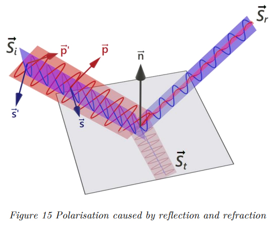
If unpolarised light hits a surface at an oblique angle, the s-polarised components will be reflected significantly stronger. Conversely, the refracted beam will be predominantly p-polarised. The effect is often explained by the fact that the incoming radiation excites dipole oscillators in the material that cannot emit radiation along their axis. However, this can be shown more generally by solving Maxwell’s equation for material interfaces demanding continuity of the electric and magnetic field at the boundary.
The calculation shows that for any dielectric material, there is a specific angle at which the ppolarised component of the reflected beam will completely vanish. Correspondingly, and taking into account energy conservation, the entire p-polarised radiation will be refracted, i.e. transmitted into the medium. This angle is called the Brewster angle. Natural, unpolarised light will be entirely polarised on reflection at Brewster angle. If, however, the incoming beam is entirely p-polarised, no reflection on the surface will occur, and the beam will be transmitted without any loss. The latter effect is exploited in photonics when the output windows of lasers are tilted at Brewster angles to suppress reflection on the windows.
Considering reflection on metallic surfaces, similar relations can be observed, though with significant quantitative deviations. Since the electrons’ movement is less restricted in metals, they generally show stronger reflection and absorption but less polarisation. Instead of the Brewster angle, a pronounced maximum for the degree of polarisation at a particular angle can be found. However, the reflected beam never reaches total polarisation.
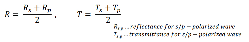
As stated above, the reflectance and transmittance coefficients are always calculated individually for the s- and p-polarised components. To get the values for unpolarised radiation, where the s- and pcomponents of the incident radiation are equal, the intensities of the reflected and transmitted polarisation components have to be averaged. The total reflectance 𝑅 and transmittance 𝑇 for unpolarised light are therefore simply determined by:

The reflectance functions for s-/p- and unpolarised incident light are depicted in Figure 16. A window glass (soda-lime glass) surface represents the dielectric case, whereas gold is chosen as a metallic surface. The calculations were performed for a wavelength of 600 nm. As can be seen, the reflection of the dielectric glass surface causes a significant degree of polarisation, reaching a value of 100% at the Brewster angle of 57 degrees. The polarisation of the light refracted/transmitted into the glass is generally lower but increases with the incidence angle to reach a value of 40% at grazing angles. The reflection off the metallic (golden) surface is stronger but generally induces less polarisation. However, the relation of the three components is similar, and while there is no actual Brewster angle for metallic materials, it can be seen that the degree of polarisation still shows a pronounced maximum at an angle of 73 degrees.

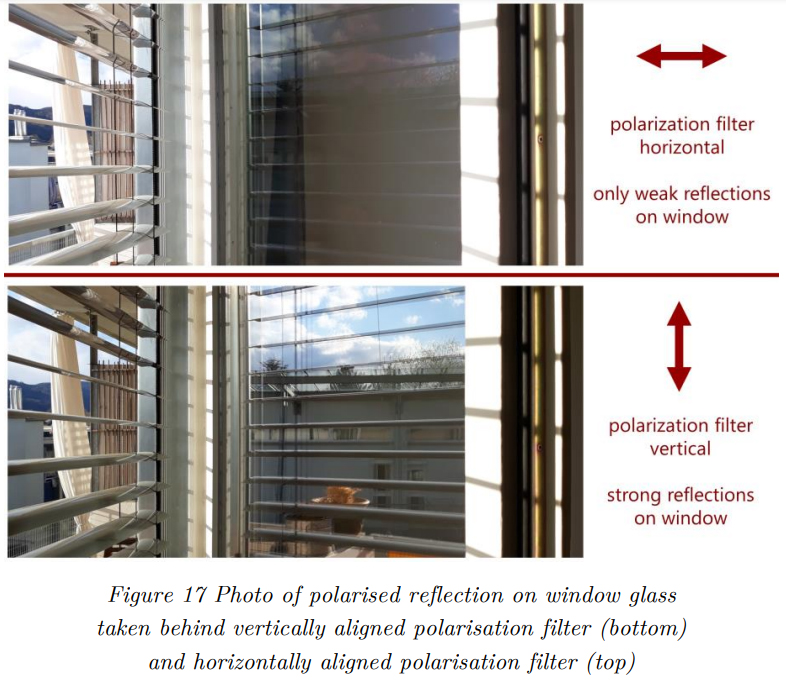
The polarising effect of reflection can easily be demonstrated if a photo of a glass surface is taken at an angle close to the Brewster angle. Since the reflected light will be almost entirely polarised, a linear polarisation filter in front of the camera can be used to filter these reflections. The effect is illustrated in Figure 17. Since the picture was taken at a close distance, the viewing angle relative to the glass changes; therefore, the filtering is pronounced at the centre of the window only.