6.1. SIOP – Solar Incidence Operator
6.1.1. SIOP concept and motivation
In order to describe the scattering characteristic of a surface (or an object comprising multiple surfaces), usually a scalar function 𝑓(𝜃,𝜑) of the zenith and azimuthal angle defined on the unit sphere’s surface is used. The scalar function then represents either the transmittance coefficients or reflectance coefficients in an angularly resolved way. However, to capture the scattering characteristics comprehensively, it is necessary to consider the direction of the incoming, as well as of the outgoing light direction. For this purpose, the concept of the bi-directional scattering-distribution-function BSDF, which is then a four-dimensional function 𝑓(𝜃𝑖 ,𝜑𝑖 , 𝜃𝑜,𝜑𝑜 ), depending on the incoming as well as the outgoing direction, is applied. In practical application, the function is either defined by an idealized analytic expression or generated based on empirical data. For the latter, the measured data is provided as discrete samples, e.g. based on the Klems-matrix containing 145×145 elements (see section 3.2). In this approach, incoming and outgoing directions are only considered on the hemispheres, as this is sufficient for most (but not all) applications.
The SIOP approach introduced here is primarily intended for energetic modelling and not for optical modelling. Therefore, the SIOP is a two-dimensional scalar function considering only the incident light’s angular distribution. Consistent with the common approaches, only the incident radiation distributed on the hemisphere (𝜃 = 0 … 𝜋 2 ⁄ ) is considered, as this will be sufficient for most practical applications.
The main objective of the SIOP definition is to overcome issues resulting from the discrete nature of sampled data. While transforming the data in the four-dimensional space of the Klems matrix into a smooth function is a hardly solvable task, the restriction of the SIOP definition to the two dimensions of the incidence light makes this much easier. Representing the scattering properties in a smooth, differentiable functional form provides significant benefits:
- integration: the SIOP can easily and precisely be integrated over any region resulting again in a smooth function (see section 6.2).
- differentiation: the smooth derivative of the function means that it can provide smooth time series at any resolution as optimal input for dynamic simulation
- interpolation: using suitable basis functions, optimal interpolation is possible
- fitting: the use of suitable basis functions allows optimal reconstruction of underlying functions that are provided in the form of “noisy” measurement samples
- data-compression: suitable basis functions allow a high level of data-compression
In the implementation, spherical harmonics have proven to represent a suitable set of basis functions for this purpose, as will be shown in the following sections. The developed method shows analogies to MP3 coding for audio data (Musmann, 2006) or the JPEG coding algorithm for images (Usevitch, 2001), as original sampled data is represented using a suitable set of basis functions.
The SIOP function can be used to determine any physical quantity 𝑞 that represents a scalar value and depends on an incidence profile 𝐼(𝜃,𝜑):

While the obvious application for the SIOP is the determination of transmitted, reflected and absorbed power using incidence profiles containing radiance information, SIOPs can also be used for other purposes. Exemplary applications of radiometry and photometry are provided in Table 10. Further applications can, e.g., involve evaluation of glare parameters, degree of polarisation, angle of polarisation, photosynthetically active radiation (PAR), colour temperature etc.

Some remarks regarding the application of SIOPs:
Time-integrated incidence profiles: Due to the linearity of light (section 4.2.2), it is always possibleto compute time-integrated target quantities when the SIOP is evaluated for a time-integrated incidence profile. This means that, e.g., total energy values for any time interval (hour, day, month etc.)can be computed within a single SIOP evaluation step if time-integrated incidence profiles for thatinterval are applied. The resulting very short evaluation times in the order of Milliseconds allow forapplying optimisation algorithms that rely on a large number of iterations.
SIOP configurations: Apart from the different dimensionality, another important difference between the SIOP and Klems/BSDF calculation method lies in the fact that for the evaluation of any SIOP, always the initial, “undisturbed” incidence profile relevant to the entire system is used. In contrast, for evaluating a system comprising multiple BSDF layers, the undisturbed incidence profile is applied only on the first layer, whereas the further layers will be evaluated using the output of the preceding layer. Therefore, the BSDF/Klems approach allows using single-layer data individually or rearranging it into new configurations. However, the approach is linked to potential sources of error in the practical application (see section 3.3). In contrast, SIOPs of any layer should only be used in the context of the system they were calculated for.
Level of detail target object: the definition of the SIOP naturally does not contain any restrictions regarding the target objects. Since the SIOPs are not based on individual layers but are generated and evaluated within the context of layer systems, they are intended to contain detailed information Solar Incidence Operators Definition, generation and evaluation RadiCal, D. Rüdisser 125 about the system. For example, the SIOPs for a window detail can and should be modelled based on a model containing details regarding its frame and/or reveal instead of only considering the glazing layers. Of course, this means that a large number of configurations has to be covered. However, by scaling the SIOP results based on a reference area, which should be contained in the description of the SIOP, it is possible to interpolate and extrapolate results using the “nearest” suitable model.
SIOP database: An intended open online database for SIOPs would allow users to share SIOPs for a wide variety of models and applications. If the models are provided with detailed information regarding their generation (model, reference area, material), they can straightforwardly be applied by any user and for any type of application.
SIOP for lighting application: on the first view, it seems that the limitation of SIOPs to a scalar value on the output side prevents the direct application of the concept in the lighting field, as directional information is usually required there. However, there are ways to overcome this limitation. The target quantity of the SIOP can, of course, also be subject to specific directional restrictions. For example, 145 SIOPs could be generated to represent the light transmitted in all directions of the KLEMS matrix. Alternatively, any other directional separation could be applied. Generally, any directional segmentation suitable for the used lighting software could be considered, e.g. separation into fewer directions, separation into diffuse and direct components only, etc. Likewise, the separation of wavelengths into any desired primary colour basis can be straightforwardly applied. However, lighting applications are not part of the present work.
6.1.2. SIOP definition and generation
6.1.2.1. Definition based on spherical harmonics
The SIOP representation relies on spherical harmonic expansion, see e.g. (Abramowitz et al., 1988; Ziegel et al., 2007). Spherical harmonics are well known for their use in quantum physics (“orbits”). As their German name “Kugelflächenfunktionen” (sphere-surface-functions) expresses, they represent a set of orthogonal functions defined on a sphere’s surface and are therefore well suited to serve as basis functions for the expansion of a general function defined on a sphere. The method is similar to the Fourier expansion of functions in 1D. Since spherical harmonics are intrinsically based on circular functions, they have proven to be very well suited for the application described here, as scattering processes are largely governed by trigonometric functions. In a general, complex-valued form, the spherical functions can be written as (Ziegel et al., 2007):

Where 𝑃𝑙 𝑚 are the associated Legendre polynomials (Abramowitz et al., 1988; Kreyszig et al., 2011). Hence, for every positive integer 𝑙 there is a subset of 2𝑙 + 1 independent functions that are iterated through by the sub-index m. Starting off with a constant function (i.e. a sphere) for l=0, the functions become increasingly complex and show an increasing number of local extrema with higher l values. As mentioned, the set of spherical harmonics possesses the remarkable (almost astounding) property of being orthonormal, i.e. the product of any two different functions will vanish, and the integral over squared function on the entire hemisphere equals one for any spherical harmonics:

For the definition of the real-valued SIOP function, it is sufficient to evaluate only the real part of the spherical harmonics, subsequently denoted here as 𝑌𝑅. Utilizing a complex conjugate identity for negative m values, the function can be written as (Sommers, 2001):

This formulation allows a straightforward software implementation. An efficient recursion formula (Ziegel et al., 2007) is used to evaluate the Legendre polynomials 𝑃𝑙 𝑚 numerically. The scaling factors 𝐶𝑙 𝑚 containing factorials (eq. (100)) are pre-computed to ensure fast evaluation. The shape of the first 12 functions is depicted in Figure 77.
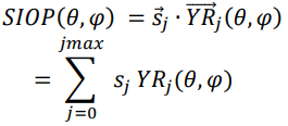
This definition allows to represent the SIOP by using a single, one-dimensional vector 𝑠 , where the coordinates of the vector 𝑠𝑗 represent the coefficients of the series-expansion. The SIOP can then be evaluated as a weighted sum of the real-valued spherical harmonics functions:


6.1.2.2. Sampling data for SIOP generation
To generate a specific SIOP for an application, such as modelling the solar transmittance of a shaded window, angularly resolved information in the form of a discrete set of sample values (𝑑 𝑖 , 𝑣𝑖) is used. The scalar values 𝑣𝑖 represent the desired quantities (e.g. the transmitted power) for light restricted to a single incidence angle, i.e. a parallel beam from the discrete direction 𝑑 𝑖 = (𝜃,𝜑)𝑖 . Although the algorithm can be performed for any set of directions, a distribution of the sampling directions with a non-regular or non-uniform pattern in an angular sense is recommended. Unlike the angular distribution of the Klems matrix (see section 3.2), a distribution with less symmetry regarding the angles is less prone to aliasing effects. Considering these requirements, the Fibonacci sphere geometry seems to provide the ideal distribution of directions for this application, as discussed in section 5.3.
The target output values 𝑣𝑖 for the sampling directions will usually be generated based on virtual measurements, applying appropriate raytracing software as proposed in this work. However, provided a suitable measurement system is available, the input data could as well be of empirical nature.
6.1.2.3. Determination of SIOP coefficients
Even though the unique property of spherical harmonics of forming an orthonormal basis would allow direct calculation of the reconstruction coefficients by integration (see, e.g. Sommers (2001) or Liu et al. (2013)), it has proven that indirect determination of the coefficients employing parameter optimisation leads to better results for the application intended here. The reason for preferring optimisation is that the measured samples 𝑣𝑖 are subject to statistical errors. Even if these errors are minor, the direct method will lead to a precise reconstruction of all samples. This means that the locally contained noise will also be reconstructed. Therefore, direct reconstruction by integration tends to generate oscillating artefacts in between the given sampling points.
Finding the coefficients based on parameter optimisation instead of using direct integration technically turns the interpolation method into a fitting method, or – ideally – into a quasi-interpolation of the unknown underlying function without any statistical errors.
In order to find this smooth, continuous representation of the measurement using real-valued spherical harmonics, the non-linear parameter optimisation simulated annealing is used (see 5.2). The stochastic method is simple to implement but has proven to be very powerful in performing global optimisations on functions that depend on many parameters and have numerous local minima (nonconvex functions).
For this application, the following cost function 𝑓𝑜𝑝𝑡 is minimised during the optimisation process:

The first factor of the cost function describes the squared deviation of the SIOP reconstruction vs.the measurement data 𝑣𝑖 and represents the main optimisation target. The second factor representsa penalty in the optimisation process that increases with the number of non-zero expansion coefficients, denoted by 𝑘. The term is not essential to the optimisation process but has proven to beuseful in reducing the amount of very small, and therefore negligible, coefficients during the optimisation. This ensures a more efficient (=faster) evaluation of the SIOP later on and tends to producesmoother representations if only little sampling information is available.
Finally, the resulting SIOP can be written and deployed in the form of a vector containing the realvalued coefficients sj of the expansion:
Since the vector usually contains mostly zero elements, it is practically more efficient to deploy (export) it in the form of an indexed array containing only non-zero coefficients ci and their indices ji (e.g. in XML or binary format):
6.1.2.4. SIOP reference system and polar
plot representation
The data contained in the SIOP can best be depicted in the form of three-dimensional polar plots. For this purpose, the actual value of the SIOP determines the radius (measured from the origin) for the two spherical angles (𝜃,𝜑) for any point on the hemisphere. By convention, the right-handed reference coordinate system for the SIOP is defined in a way that the z-axis points towards the direction of normal incidence and the y-axis is aligned to the vertical axis of the object (or any other reference axis, if not available). The xy-plane, therefore, reflects the reference plane of the object (e.g. the plane parallel to glazing). For consistency, any SIOPs should be generated using this orientation.
The z-axis, which points towards the direction of normal incidence to the reference plane, also represents the main symmetry axis for the evaluation of the spherical harmonics (corresponding to 𝜃 = 0°), whereas the azi

muthal angle 𝜑 is defined on the xy-plane. The polar plot representation for the SIOP and the reference axis and angles are depicted in Figure 78 (the exemplary SIOP represents the transmission through a shaded window with 30° tilted blinds).
6.1.3. Implementation
All data representing a SIOP is contained in the class TRCSIOP of the module rc_siop. The class TRCSIOP contains an instance of the class TFibonacciSphere that is initialised with the number of directions (ssNDir) representing the sampled angular distribution. This means that the sampling directions are not stored in the file but are regenerated using TfibonacciSphere. The class TRCSIOP also includes an instance of the class TSphericalHarmonics that provides the algorithms necessary to evaluate the spherical harmonics according to equations (103). Further, it temporarily contains the azimuthal and tilt angle of the SIOP used for the most recent evaluation process, as well as the associated vector transformation matrix.

All permanent data defining a SIOP, which is usually stored in a file, is structured in the TSiopData class. It covers the following information:

The class contains three types of information:
- sampling data: the original sampled data, that is usually determined in the virtual measurement, i.e. raytracing process or alternatively using empirical methods. This original data is always kept within the SIOP. The information can be used for extended analysis or regeneration of the functional form. Further, supplemental information regarding the source of the sampling data is contained here (e.g. target object name, reference area, type of SIOP etc.).
- functional data: this part contains all information required to construct/evaluate the functional form of the SIOP.
- cached evaluation data: variables necessary for evaluating a SIOP are stored here (see section 6.2.4). Since this data is mainly generated using numerical integration, it is cached in the SIOP. Reusing values computed on earlier occasions increases the performance of later evaluations with the same tilt angle. The data contains the orientation and coefficients of the most recent evaluation.
To actually evaluate a SIOP in a simulation run, the evaluation has to be initialised by calling initSIOPorientation (to define the SIOP orientation in the real-world coordinate system) and precalcHemiMeans to initialise the constants used for evaluation (see next section).
After that, the function evalSIOPWorld will return the value of the SIOP for any desired direction:

The evaluation of the spherical harmonics series is performed in the function evalSIOPStdSYS:

The coefficients of the spherical harmonics (equation (103)) are provided by the function Ysh function, which is implemented in the module TSphericalHarmonics.
The determination of the coefficients based on the simulated annealing optimisation method is performed by the class TRCSIOPanneal in the module rc_SIOPanneal.
The method anneal is called with the relevant parameters to convert any given SIOP samples into the functional form.

6.1.4. Exemplary generation of SIOPs
In order to allow a better understanding of the method and to prove its efficiency, an exemplary application is provided here. The application does not focus on the quantitative results, as this is covered in later chapters. Instead, this example should demonstrate the process of SIOP generation. Four SIOPs describing the direct transmission of a fenestration detail comprising a triple-glazed insulated glass unit (IGU) shaded by external Venetian blinds, are generated. In the example, the state “unshaded window”, as well as the states “fully-shaded” with three different slat angles, are analysed. Based on the nature of the method, the evaluation also includes any reflections with the reveal or on the window sill. To gen

erate the measurement samples for the SIOP generation, a (here unspecified) raytracing algorithm is applied to a detailed CAD model of the fenestration (Figure 79). Provided a suitable measurement method is available, the samples could also be of empirical nature. In this example, 1444 equally spaced sampling directions of the Fibonacci-hemisphere (see section 5.3) are used to measure the effect of different parallel-beam incidence profiles on the physical quantity of interest. In the case presented here, the power transmitted to the internal of the building is analysed.

The sampled measurements are converted into SIOPs using the method described above. The annealing process for each sampling set, which determines the optimal reconstruction coefficients, lasts for about 15 minutes each (on a single average CPU). Each optimisation iterates through approxi
mately 30 millions possible configurations. The available base of spherical harmonics has been restricted to 440 potential base functions by setting lmax=20. The quality of the resulting reconstructions is quantified based on the absolute mean errors for the individual samples and the mean errors weighted by the (almost identical) solid angles for each sample. Geometrically this also corresponds to the volume of the SIOP if it is represented in polar plot representation (see Table 11), as the solid angles represented by the samples are almost equal (see section 5.3).

Remarkably, the reconstruction’s mean error (or total volume error) is exceptionally low, i.e. by several orders of magnitude lower than the absolute mean error for each sampling point. The higher mean absolute error is also a result of the somewhat “noisy” input data. As the samples are the results of a stochastic raytracing process, they are subject to a certain degree of statistical errors (see 5.1.3). However, since the (signed) mean error (or total volume error) is not an explicit optimisation criterion, the excellent match regarding this measure indicates that the spherical harmonics can

capture the geometric nature of the underlying process rather than only reconstruct the individual samples. The high data compression rate also supports this interpretation: the information of each case, represented by 1440 sampling points, can be reconstructed by summation of less than 90 spherical harmonics, as shown in the first row of Table 11.
The polar plot representations for the sampling data as well as for the final functional SIOP, are depicted in Figure 81. It can be seen how the final shape of the SIOP matches the sampled data. The polar plots presented in Figure 82 reveal the directional dependencies of the different shading states. The unshaded state is open to a broader angular range with a peak at normal incidence. Note that the ideal case of a simple planar absorber, governed only by the cosine law, would result in a perfectly spherical SIOP. However, due to the shading effects of the window reveal and the angular characteristics of the glazing, the SIOP of the unshaded window detail shows a rather balloon-like shape with smaller values for higher angles of incidence.

Once the shading is closed, maintaining horizontally oriented slats, the SIOP is squeezed towards a lentil-like shape, as predominantly light from relatively horizontal directions can pass the blinds. Compared to the unshaded state, the hemispherical mean value of transmittance is reduced to 57% for the horizontal (0°) slat angle, as can be seen in the polar plot by the decrease in size. Tilting the slats further reduces the hemispherical mean value to 24% (for 30° tilt) and 6%, respectively (for 60° tilt). It can also be seen how the direction of maximum transmission is tilted along with the slat angle.