5.2. Simulated annealing

actually quite astounding that trillions of molecules or atoms can arrange themselves in a way that their macroscopic arrangement reflects an energetically ideal shape. How is this possible? The answer to this question is the principle behind the simulated annealing optimisation algorithm: Firstly, excess energy determined a temperature measure is provided to the system to allow an efficient reconfiguration of its constituents. These reconfigurations also include transitions to energetically less optimal configurations. Second, the temperature, i.e. the associated excess energy, is slowly reduced, and the probability for less ideal configurations decreases along with it. In order to determine what configurations are possible in such a process, first some funamentals of thermodynamics, or statistical mechanics to be more precise, have to be considered. At thermal equilibrium the probability that a system with N potential states can be found in the state i having energy 𝐸𝑖 , is described by the Boltzmann distribution:

Metropolis proposes an efficient way to populate these states numerically in his publication (Metropolis et al., 1953). In order to generate configurations matching the Boltzmann distribution, the following strategy is applied:

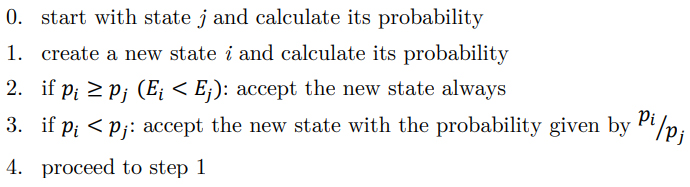
If the temperature is gradually reduced during this process, the system moves effectively to its ideal state, as the temperature dependence of 𝑝𝑖 𝑝𝑗 ⁄ increasingly rules out less ideal states (see Figure 70). However, since at higher temperature levels, less optimal configurations are still accepted, it can be avoided that the optimiser gets trapped in local minima early. If the annealing process were given infinite time, it would reach the optimal solution, i.e. the absolute minimum of the cost function, as it would escape from any local minima again. In its practical application, with limited processing time, it cannot be guaranteed that the ideal state can be identified. However, simulated annealing is able to identify good solutions for such problems very efficiently.
In its practical implementation, the following four components need to be implemented to perform a simulated annealing optimisation (see, e.g., Ziegel, et al. (2007), Penna (2002)):

1. Definition of a state

A concise and unambiguous structure containing all state parameters of the system has to be provided.

2. Cost function

A function that is used to evaluate the optimality of a state (its “energy”). The target of the optimiser is to find the absolute minimum of this function. Often the function is defined in negative values. However, only the difference between two evaluations of the cost function is considered in the algorithm. Therefore, its absolute value is irrelevant.

3. Alteration algorithm

An algorithm that is able to generate random new states is necessary. This function has a significant impact on the efficiency of the optimisation. While it is generally possible to create new states independent of the current state, it proved that an algorithm that is able to generate incremental adaptions of the current states is more efficient for most problems. Generally, a combination of both is applied.

4. Temperature and cooling schedule

Following the thermodynamic fundamentals, the cooling schedule usually provides a logarithmic temperature decay. However, the actual cooling schedule depends on the cost function and the nature of the optimisation task. In most cases, “phase changes” in the system can be observed. These represent temperature regions where the cost function remains constant to drop sharply afterwards. Since this implies that the system transitions into a path of new configurations, making it harder to access previous states, it is advisable to slow down the cooling at such critical temperature ranges. This can, e.g., effectively be achieved by tracking the average costs with two exponential moving averages of different period lengths. If the deviation of the two measures indicates a sharper decrease, the cooling speed should be reduced, whereas it can be increased if the ratio of the averages indicates little change.

In order to demonstrate how simple the core of the annealing algorithm is, a simple example is provided below. All applications of the algorithm used in this work follow the presented scheme. Only the usually applied additional features to adjust the cooling schedule dynamically are omitted below for reasons of clarity.

As can be seen, the algorithm described above can be simplified to calculating the difference of both cost functions and using it to determine the probability for a new, energetically less optimal state by calculating the probability exp(-delta/T) as this is equivalent to the ratio 𝑝𝑖 𝑝𝑗 ⁄ .