Subsurface scattering
4.11.1. Background and theory
In many rendering approaches, a three-component model is used to approximate the optical behaviour of surfaces. It involves specular reflection, diffuse surface reflection and diffuse subsurface reflection (see Figure 50).
Specular reflection directly results from solving Fresnel’s equations for flat surfaces. Diffuse reflection on the surface occurs due to its topology, i.e. roughness. In the RadiCal approach, microfacet models are used to model this effect. Therefore, the specular (A) and diffuse surface (B) reflection on the surface are implicit parts of the extended Fresnel model, and the relevant dependence on roughness and incidence angle arises intrinsically. This approach also allows considering the presence of thinfilms on the surface.

Subsurface reflection (case C), however, has to be covered by an additional model. Subsurface reflection results from light rays penetrating through the (rough or flat) surface. If the material below the surface is a conglomerate showing a spatial variation of refractive indices, then the incoming light will suffer multiple scattering events, and finally, a fraction will exit beyond the surface again. The effect is, therefore, also referred to as ‘subsurface scattering’ or ‘volume scattering’. Materials with significant subsurface scattering are sometimes called translucent to express that they are neither transparent nor opaque. Common materials with strong subsurface scattering are wax, milk, skin, leaves or minerals. These materials allow relatively deep penetration of light below the surface. However, in many materials, subsurface scattering occurs directly below the surface.
For the indented technical application of the raytracer, paints represent the probably most relevant type of material requiring the modelling of subsurface scattering. Paints are made of a binder containing small particles referred to as pigments. Binder materials, e.g. oils, resins or gums, generally are transparent and have a low refractive index to allow the light to penetrate below the surface. In contrast, pigments exhibit very high refractivity in some parts of the spectrum and effectively scatter light of the corresponding wavelengths while other parts of the spectral range are absorbed. The Monte Carlo raytracing approach applied in the RadiCal method allows a detailed simulation of multiple scattering events within the volume of an object. This enables the implementation of specific models for a variety of layered or homogeneous translucent materials. In this first version, however, a simpler approach has been implemented.
Based on a given spectrally resolved subsurface reflectance function 𝜌𝑠𝑠, it is assumed that a fraction of light refracted below the surface is diffusely reflected to the outside again. This first implementation assumes a perfect diffuse directional distribution according to a Lambert reflector (see section 4.3.3). Further, it is assumed that the multiple scattering events lead to a full depolarisation of the reflected light. The two assumptions are approximations that are often applied. The Light, sun and optics – applied principles, models and methods RadiCal, D. Rüdisser 90 implementation of the ideal diffuse and depolarised subsurface reflection, therefore, allows modelling surfaces in line with many existing approaches, including the current ISO standard approach for modelling shading devices.
Additionally, more refined subsurface scattering models can be integrated in the future. The potential extension of the scattering models can be divided into two groups. On the one hand, commonly used BRDF scattering models, like the widely used Oren-Nayar model (Oren and Nayar, 1994), can be added. However, it has to be considered that many effects that these models are based on are already covered by the microfacet approach. On the other hand, following the raytracing approach, new subsurface models could comprise explicit subsurface scattering models and consider effects occurring when the potentially rough surface is passed again from the backside. This approach would also allow tracking the reflected light’s polarisation state.
4.11.1.1. Sampling the outgoing direction on a Lambert surface
The subsurface reflectance module needs to provide an outgoing direction for the reflected ray following the principles of Lambert reflectance. While the BRDF function of a Lambert surface, being constant throughout the hemisphere (see section 4.3.3), might indicate uniform sampling of the hemisphere, sampling from the perspective of radiance must be considered. Following the Lambert assumption, it is evident that the directions on the hemisphere must be sampled with a cosine weighting, as directions near the surface normal will contribute stronger.
In order to obtain this distribution for the direction of the diffusely reflected light, the inversion method (see section 5.1.2) is applied to determine the 𝑧-coordinate. The 𝑃𝐷𝐹 that has to be proptional to 𝑐𝑜𝑠 𝜃 is integrated and subsequently inverted to obtain 𝐶𝐷𝐹−1 . The 𝑥 and 𝑦 coordinates are determined by equally distributed points on the corresponding circle of the hemisphere. Two independent random numbers 𝑢1 and 𝑢2 are used in this process.

The actual implementation follows this method; however, some numerical optimisations are appliedto increase the algorithm’s efficiency (see next section).
4.11.2. Implementation
In analogy to the refractive index module, an abstract base class for the subsurface scattering function, which provides the subsurface reflection as a function of wavelength, is defined and inherited to child classes, which carry the specific models. Currently, three different models are available; additional models can be implemented straightforwardly.

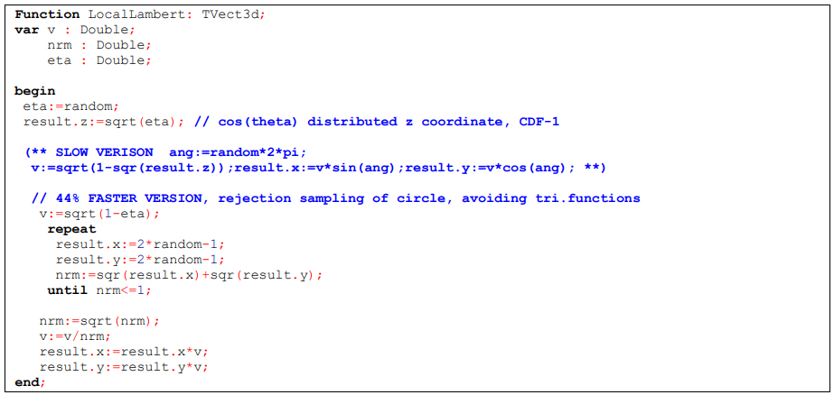
The class TssRhoConst allows the definition of a constant subsurface reflectance value for the entire wavelength range (grey or white material). The class TssRhoSpline can be used to define reflectance values based on spline functions with a variable number of knots. Currently, mainly this class is used as it corresponds to the reflectance behaviour of pigments, which usually show smooth and continuous variation rather than edges. Finally, to be able to import tabulated data, the TssRhoTableLinIP is available. It allows describing the reflectance curve using linear interpolation between given points. In order to generate the outgoing direction, a unit vector aligned to the local system (where the zaxis equals the macroscopic surface normal) is generated. The implementation follows equation (74); however, to avoid the time-consuming sine and cosine function calls the random points on the circle, providing the x- and y-coordinates are generated using a rejection sampling method. The approach is based on an algorithm commonly referred to as ‘Malley’s method’ (Malley, 1988). The implementation was found to be 44% faster than the original algorithm. In the algorithm, firstly, a random point within the unit square is chosen. If this point lies within the unit circle, its coordinates are scaled to match the radius of the unit sphere; otherwise, a new point is processed. This method provides points that are equally distributed on a circle.
4.11.3. Testing and validation
In order to test the LocalLambert function, some basic statistical tests are performed on the distribution of the directions provided. The function is called for one billion times generating samples to perform two statistical tests. Firstly, the mean vector of all samples |𝑣 𝑖 | is calculated. Additionally, the result is segmented into one million subsamples of sample size 1000 to analyse the validity and convergence of the three coordinates of the mean vector.
The calculation results for the average coordinates and standard deviation are:

For the cosine-weighted hemisphere, the mean value is expected at (0,0, 2 3 ⁄ ), which can be shown by integration. In addition to that, the central limit theorem (see section 5.1.3) is applied to check for an error or bias in the result. For this purpose, the statistical error that has to be expected for the given number of samples is determined. Applying equation (91), the standard error of means for the three coordinates are:

Therefore, the deviations of |𝑣 𝑖 | are well within the range that can be expected statistically. No bias or error in the results is detected.
For the second test, a histogram of the results is created to validate the cosine dependence of the directions. If valid, the density of the random directional samples has to increase with the cosine of the angle between the given direction and the surface normal vector. Since the generated directions are aligned to the local surface plane with 𝑛⃗ = (0,0,1) and the angle between the direction vector 𝑣 and 𝑛⃗ can be written as 𝑣 ∙ 𝑛⃗ = (0,0, 𝑣𝑧 ) = 𝑐𝑜𝑠 𝛼, a linear relationship between the density of the random directions and their z coordinate is expected. In order to test this, a billion directional samples were compiled in a histogram with 100 bins using the z-coordinates for classification.

As shown in Figure 51 and Figure 52, the almost perfect correlation of the distribution of sampled directions with the z-coordinates confirms the cosine dependence and, therefore, the validity of the implemented Lambert algorithm.