5.3. A Fibonacci hemisphere
5.3.1. Background and theory
In the method presented here, the scattering or absorption behaviour of the analysed system is not provided in a discrete form (like the Klems matrix) but in a functional form. However, in order to derive this functional form (SIOP, see section 6.1) it is necessary to provide discrete measurement samples of the target quantity for different incidence directions on the hemisphere. The most suitable distribution of incidence directions for the intended technical application should cover the hemisphere with equal spacing. A regular angular pattern, as provided by the Klems segmentation, does not seem ideal for that purpose. The reason for that is threefold: first, the two-axis symmetry (vertical/horizontal) of the angular Klems pattern will often lead to an inefficient sampling of
redundant information, as the analysed object (e.g. shaded window), will often also show symmetryin the vertical and/or horizontal axis. In the case of a rotationally symmetric behaviour (e.g. ofunshaded glazings or textile screens), the full Klems matrix can be derived from only nine incidencedirections. Second, the regular spacing of the two angles is more prone to sampling issues, e.g.aliasing, since the analysed applications, like a window shaded by tilted Venetian blinds, will alsoshow a pronounced regular angular pattern. Sampling this angularly equally spaced pattern at a fewequally-spaced detection angles can easily lead to aliasing effects if these patterns are correlated.Finally, the angular resolution of the Klems matrix decreases for higher incidence angles 𝜃 and istherefore less able to capture gradients of shadings or reflectivity increases that are dominant atthese angles (see below).
Following these arguments, it seems more appropriate to distribute the sampling directions evenlyon the hemisphere with little symmetry regarding its angular distribution. Providing an even distribution of directions (points) on a sphere is a theoretical topic with a long history and high relevancein various scientific disciplines.
Various approaches are available for that purpose, like the icosahedron algorithm and numerousmethods based on numerical optimisation. Considering all requirements stated above, the Fibonaccisphere method seems to provide the ideal distribution of directions here:
- a) it provides an almost perfect evenly spaced distribution on the sphere (hemisphere)
- b) it shows little symmetry regarding the vertical or horizontal axis
- c) it can be generated for any desired number of sampling directions N
- d) it is a direct and fast method (as it is not based on optimisation)
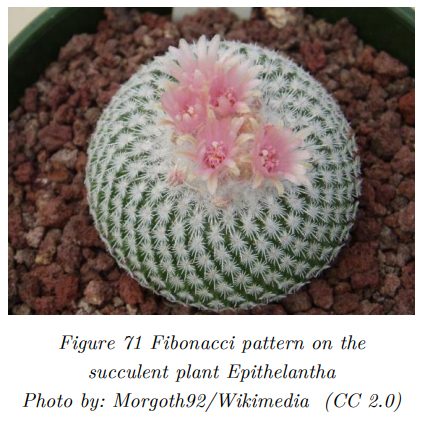
The angular or spatial patterns that are based on Fibonacci distributions are frequently found in nature, for example, the arrangement of seeds (e.g. sunflowers) or leaves (e.g. aloe plants). The frequent occurrence in nature is generally a good indication regarding the efficiency and optimality of the distribution.
5.3.1.1. The Fibonacci sphere algorithm
In order to derive a Fibonacci sphere, firstly, a Fibonacci lattice on the unit square is considered. The coordinates for the corresponding vertices 𝑝𝑖 can be written as (Marques et al., 2013):
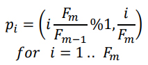
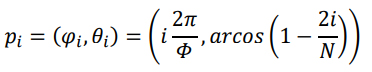
Where 𝐹𝑚 and 𝐹𝑚−1 are the elements of the Fibonacci number series, and % stands for the modulo operator. Using a Lambert cylindrical equal-area projection, the pattern can be mapped on a sphere. Additionally, the ratio 𝐹𝑚 𝐹𝑚−1 is substituted with the golden ratio 𝛷 = 1 2 ⁄ (1 + √5), as the ratio of consecutive Fibonacci numbers quickly converges to this ratio for higher 𝑚 values (Graham et al., 1994). Consequently, the vertices for a Fibonacci sphere with 𝑁 = 𝐹𝑚 elements can be expressed in polar coordinates as

5.3.1.2. A (slightly) optimised Fibonacci hemisphere
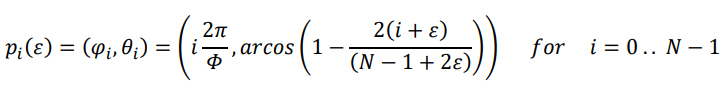
This canonical Fibonacci distribution can be optimised by inserting an offset ε at the beginning and the end of its vertical distribution (94). Further, the distribution is shifted in a way that it is symmetrical in its z coordinates, as the original distribution has its top vertex slightly offset (𝑧 = 2/𝑁) and its bottom vertex at the bottom pole (𝑧 = −1). Hence, the z coodinates of the 𝑁 points, that are initially equally spaced within the interval [−1, 1 − 2/𝑁], are now mapped onto the interval [−1 + 𝜀, 1 − 𝜀]. The distribution of the directions in polar coordinates can then be written as:
In Figure 72, it can be seen how the first vertex is offset from the pole along the helix formed by the vertices. The vertical distance of this offset is defined by the parameter 𝜀. The parameter 𝜀 can now be used to “fine-tune” the distribution of the directions. Deviating from the proposal made by Roberts (2020), a constant value 𝜀0 for all 𝑁 values is sought here. This shall, on the one hand allow simple replicability of the distribution and on the other hand the value of 𝜀 converges quickly for – the here relevant – higher 𝑁 values anyway. The maximization of the average minimum distance 𝛼̅ of all vertices has been chosen as the criterion for the optimisation process:
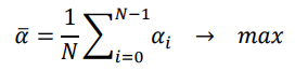
with 𝛼𝑖 being the minimum angle between the vertex 𝑖 and its closest neighbour. Additionally, since – for the application intended here – only the hemisphere is considered, a new constant 𝑁ℎ𝑒𝑚𝑖 is introduced. 𝑁ℎ𝑒𝑚𝑖 represents the number of Fibonacci vertices that are provided for the (upper) hemisphere. However, 𝑁ℎ𝑒𝑚𝑖 does not need to be identical with the half of the 𝑁. Rather, for any desired 𝑁ℎ𝑒𝑚𝑖, 𝑁 is determined in a way that precisely 𝑁ℎ𝑒𝑚𝑖 vertices of the upper hemisphere are located above a certain threshold ξ. This threshold value is introduced to avoid grazing incidence angles, i.e. almost parallel directions. These grazing directions can be detrimental, as they can increase the calculation time
or lead to numerical issues. The height threshold value, which applies to the cosine of 𝜃 (=z-coordinate), has been defined as ξ = 0.001.
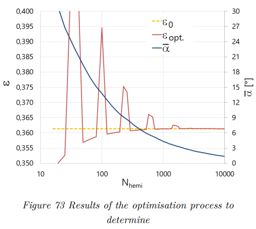
In the optimisation process, the optimal values for 𝜀 according to equation (96) for hemispheres with an increasing number of directions 𝑁ℎ𝑒𝑚𝑖 (up to 10,000) were analysed. The results of the optimisation process are depicted in Figure 73. It can be seen that while there are different solutions for smaller 𝑁ℎ𝑒𝑚𝑖 distributions, the value of 𝜀 converges for higher numbers. Therefore, a constant value of 𝜀0 = 0.3613 is defined and universally applied in the following.
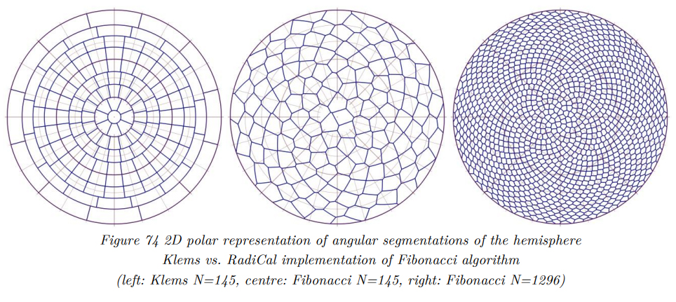
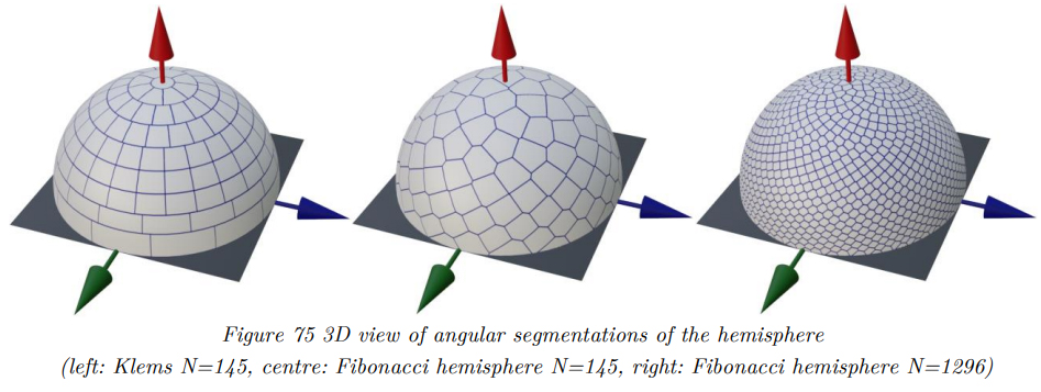
. Figure 74 and Figure 75 show the angular segmentation of the hemisphere according to the classical Klems approach and the implemented Fibonacci approach as polar plots and 3D representations. As can be seen, the Klems matrix shows high symmetry in multiple axes as well as angular correlations. Both features are not ideal for the RadiCal approach. By contrast, the Fibonacci segmentation shows no axial symmetries and little correlation. It can also be seen that due to the actual implementation, the first Fibonacci patch is slightly offset from the pole, which is intended.
5.3.1.3. Analysis of distributions
In order to analyse the quality of the angular distributions, the corresponding solid angles are analyzed. For the Klems segmentation, these are explicitly provided in its definition, while for the Fibonacci hemisphere, they are computed based on a proximity criterion. The solid angles of the Klems distribution show a significant variation due to the regular segmentation in 𝜃. The solid angles of the angular patches increase with the incidence angle 𝜃. This was obviously a design choice of Klems, as the relevance of these directions
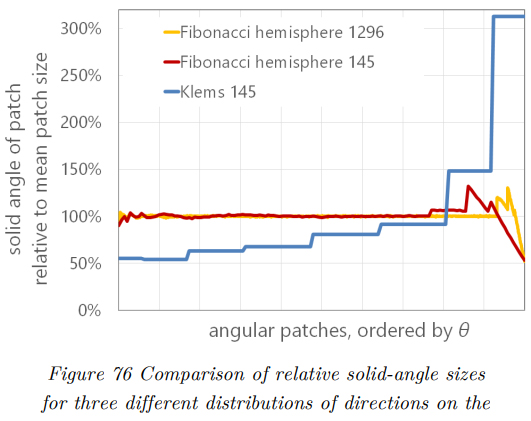
will, for many applications, usually decrease proportionally with 𝑐𝑜𝑠(𝜃). On the other hand, it can be argued that higher gradients of the represented functions (such as the transmission of the window) can be expected mainly for these higher incidence angles. For example, the area shaded by protruding parts or the reveal will increase proportionally to 𝑡𝑎𝑛(𝜃). Hence, correctly capturing this characteristic requires higher sampling resolution for higher incidence angles. Considering both arguments, sampling with equally spaced directions, as provided by the Fibonacci hemisphere, seems to be the most appropriate approach. Figure 76 shows a comparison of the solid angles that correspond to the angular patches provided by three different distributions. It can be seen that the patches of the Klems distribution for the highest incidence angles (>75°) are approximately six times larger than the ones near normal incidence (0°). In contrast, the Fibonacci distributions provide almost perfect equally-spaced directions for most incidence angles. Only in regions near grazing incidence (close to 90°) a fluctuation of the patch sizes is apparent. The reason for this is the clipping effect by the surface plane and the threshold height criterion.
5.3.2. Implementation
In the implementation, all algorithms relevant for setting up and evaluating the Fibonacci hemisphere are contained in the class TFibonacciHemiSphere of the library rc_fibonacci_sphere.
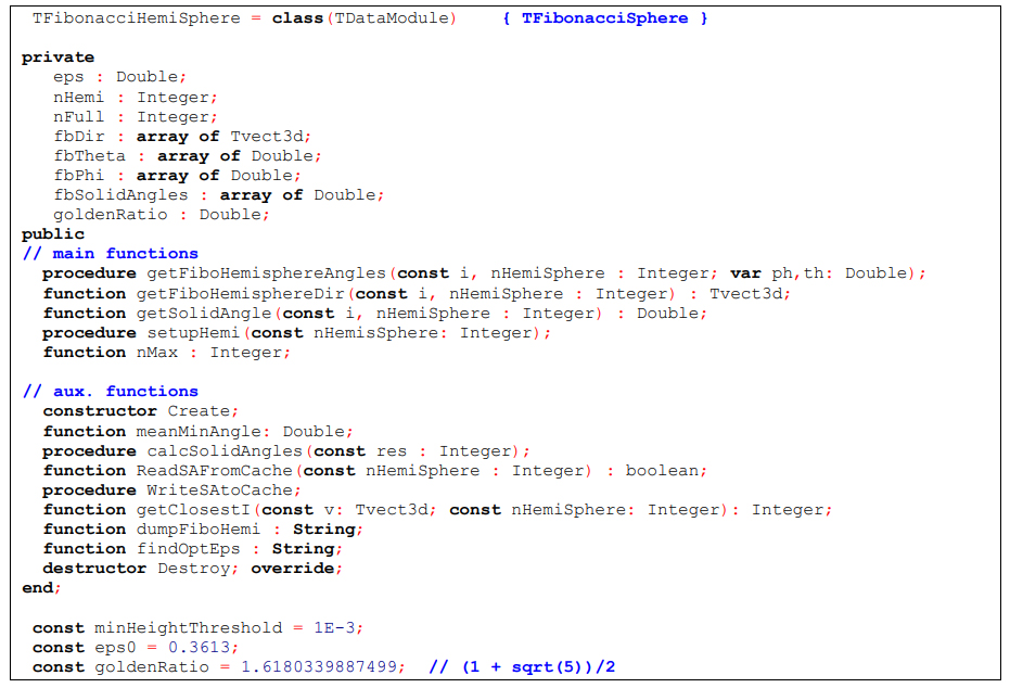
The angular and vector-based data is precomputed to increase performance. The precalculation can either be performed directly by calling the procedure setupHemi or indirectly by calling getFiboHemisphereAngles or getFiboHemisphereAngles for the first time, as they will, in turn, call the setup procedure.
The actual and remarkably simple Fibonacci algorithm is contained in the setup procedure. It is presented in full here:
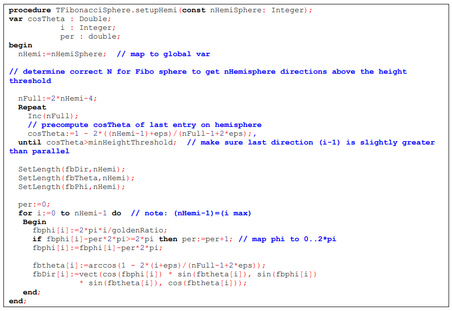
In the first part of the setup procedure, the correct value for the number of directions on the entire Fibonacci sphere 𝑁 is determined. 𝑁 is determined in a way that ensures that precisely the desired 𝑁ℎ𝑒𝑚𝑖 are located above the height threshold. Afterwards, the angles and vectors that define the 𝑁ℎ𝑒𝑚𝑖 directions are precomputed based on equation (95) and stored in the corresponding arrays.
5.3.3. Testing and validation
During the implementation of the algorithm and, in particular, during the optimisation of the parameter 𝜀0 several tests and validations of the algorithm were performed. The distribution of solid angles and angles among the directions were computed and analysed for many different 𝑁ℎ𝑒𝑚𝑖 values. Beyond that, the visual representations, as depicted in Figure 74 and Figure 75, are a reliable indicator for the validity of the implemented code.